Serial killer: Drawdowns and serial correlation

Drawdowns. You hate them. I hate them. Where do they come from? Here are two of the usual suspects:

(1) μ = mean returns

(2) σ = return volatility

The standard view is that drawdowns occur when you have either low μ or high σ or both. For example, the U.S. stock market reached a drawdown of about 50% in February 2009. The standard view says that this GFC drawdown reflected high realized volatility and low average returns. Of course, the GFC was a complicated series of events; μ and σ are just statistical measures we use to describe the underlying reality.

μ and σ are vital building blocks in finance. We can use them as forward-looking concepts to describe our beliefs about the future, or as backward-looking concepts to describe realized returns in a particular sample period. We all spend a lot of time trying to analyze and predict μ and σ, and there’s nothing wrong with that. But there’s a third perpetrator of drawdowns that’s often overlooked:

(3) ρ = first-order serial correlation of return (a.k.a. autocorrelation).

Positive serial correlation leads to bigger drawdowns, while negative serial correlation leads to smaller drawdowns. If you have two strategies with the same Sharpe ratio but different ρ, the strategy with higher ρ is riskier and has higher expected drawdowns.

First-order serial correlation is one of many ways to describe temporal dependence in returns; another good choice is the variance ratio as in Lo and MacKinlay (1988). But for simplicity, let’s stick with ρ. Asset returns are typically close to random, which means that monthly ρ is typically close to zero. The usual method of annualizing monthly standard deviations (just multiplying by the square root of 12) is appropriate when ρ=0, but when ρ>0, this method will understate true annual volatility.

There’s a common belief that the main threat to your wealth is a huge one-day or one-month crash, a left-skewed “tail event” that will destroy your wealth in the blink of an eye. That outcome happens sometimes, but it’s not how the world usually works. Usually, disaster manifests as a sequence of bad days that sum up to a sequence of bad months, as opposed to one gigantic bad day. Your main concern should be a slow bleed, not sudden death.

Numerical example

The drawdown of an investment is defined as the current value minus the trailing maximum value, expressed as a percent of the maximum. To illustrate its properties, let’s take a simple example. Suppose we have an asset that each year has returns of either +20% or -10% with equal probability. This asset has μ of +5% and σ of 15%, so it has a return profile similar to the stock market.

To make things simple, let’s suppose that over the next ten years, we know for certain that the asset will have exactly five up years and five down years; there is only uncertainty about the sequence in which the up and down years appear. So, we’re assuming that for sure, μ is 5% over the next 10 years. While this assumption is unrealistic, it allows us to focus on just the sequence of yearly returns. This assumption means that if we invest $100 at the beginning, after 10 years we’ll have $147 no matter what. At a 10-year horizon, this asset is riskless given our assumptions, and long-term holders don’t need to worry about the sequence of returns.[1]

While a truly locked-in long-term holder isn’t impacted by the sequence of returns, the asset is not riskless if we might need to sell it before 10 years have elapsed. In that case, we care very much about the sequence of returns and the maximum drawdown that may occur.

Let’s take two extreme cases. First, ρ = -1, and each up year is invariably followed by a down year and vice versa. Second, ρ = +0.8, where the up and down years always appear five-in-a-row. Figure 1 shows the drawdowns arising from the worst-case scenario for both.

In the case of negative serial correlation, the maximum drawdown will be -10% and it’s possible that we’ll put in $100 but only get $90 back. If we stay invested over 10 years, we’ll always gain $47, but if we need to bail after only one year, we might lose $10. In the case of positive serial correlation, the maximum drawdown will be -41%, and we might lose $41 if we get five down years immediately after investing.

Figure 1: Numerical example – Effect of Serial Correlation on Drawdowns

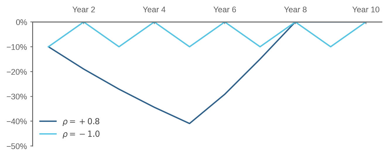
Positive ρ is a serial killer of wealth. Negative ρ is a helpful friend. Figure 1 shows that ρ causes drawdowns.

Of course, here I’m anthropomorphizing ρ for dramatic effect; we all understand that ρ is actually not a person but instead is just a descriptive statistic that summarizes the underlying data. Similarly, I’m exaggerating when I say that ρ “causes” drawdowns; it is the clustering of returns that causes drawdowns, and ρ just measures the clustering.

So when I say that ρ causes drawdowns, that’s just shorthand for the more unwieldy statement that “drawdowns are the result of the realized sequence of returns in calendar time reflecting some mixture of random chance and the temporal dependence in returns inherent in the underlying and possibly time-varying data generating process.”

How important is ρ? Looking at monthly simulations, Van Hemert et al. (2020) show that higher serial correlation produces higher drawdowns and calculate that the increase in drawdowns generated by raising monthly ρ from zero to +0.1 is equivalent to lowering the Sharpe ratio from 0.5 to 0.4. As an empirical matter, Daniel, Hodrick, and Lu (2014) argue that:

Adding conditional autocorrelation, especially in down states, seems necessary to fully characterize the distributions of drawdowns …

In the next section, I show that for U.S. stock returns, ρ is quite impactful and going from a positive ρ to a negative ρ would greatly decrease the drawdown during the GFC.

Drawdowns in the aggregate U.S. stock market

Figure 2 shows monthly data for the CRSP aggregate stock market index from January 2000 to June 2025, from the data library of Professor Ken French. The solid line shows the trailing 60-month ρ of monthly returns, while the dashed line shows drawdowns.

Figure 2 shows wide variation in realized ρ. The average ρ is +0.02 over this period, but trailing 5-year ρ gets as high as +0.4 in the GFC and as low as -0.26 in 2016. While we can argue whether this variation is merely random ex post, and whether it might be predictable ex ante, it is clear that realized ρ moves around a lot.

Figure 2: U.S. Cap-Weighted Market – Drawdowns and Serial Correlation

Since 2000, the U.S. stock market has experienced two major drawdowns, the first in 2002 after the unwinding of the tech-stock bubble, and the next in 2009 during the GFC. Figure 2 shows these drawdowns had very different statistical properties. The 2002 drawdown was accomplished by μ and σ alone, without the assistance of ρ which hovered around zero in this period. But the GFC drawdown was aided and abetted by a high positive ρ.

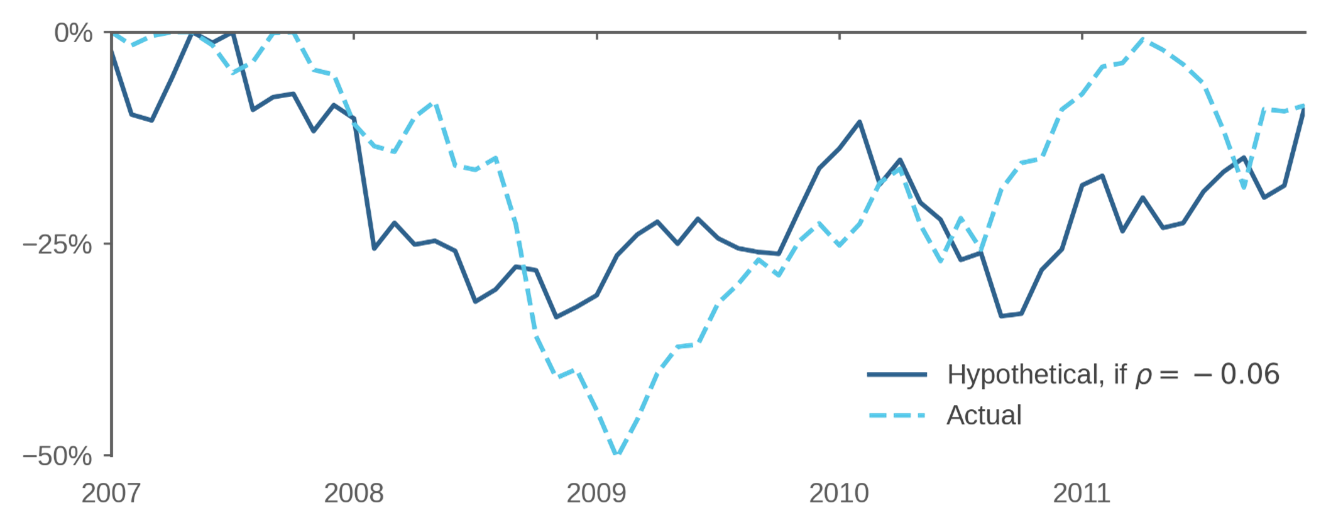
Figure 3 explores the impact of ρ on drawdowns around the GFC. The dashed line shows the actual drawdown of the aggregate U.S. stock market from 2007 to 2011, the same line shown in Figure 2. During this five-year period, ρ was +0.22, and this positive serial correlation partly explains the drawdown of -50% in February 2009.

How bad would the GFC have been if we could have magically flipped the sign of ρ during this period? The solid line in Figure 3 shows the drawdown that results from rearranging the 60 monthly returns between January 2007 and December 2011 so that ρ is -0.06 instead of +0.22. As in Figure 1, both lines in Figure 3 use exactly the same returns with exactly the same μ and σ.

The maximum drawdown with negative ρ is now -34% instead of -50%. While Figure 3 only shows one return sequence out of many possible counterfactuals, the point is that μ and σ are not the only culprits in explaining why the GFC was painful. With ρ of -0.06, the GFC might have been a less traumatic experience for equity investors.

The period from 2007 to 2011 featured a complicated series of events involving financial markets, government actions, the revelation of information over time, and possibly self-fulfilling expectations by market participants. My point is that ρ is a useful way to describe these events. It is not enough to say that stock returns were very volatile in 2008/2009; to describe the GFC, you need to capture the fact that we experienced a sequence of bad returns.

Figure 3: U.S. Market Drawdowns – Actual and Hypothetical

So my view is that, for any given return frequency and sample period, drawdowns are caused by some combination of the following three things: μ, σ, and ρ. Of course, it is possible to get drawdowns without requiring the involvement of σ or ρ. For example, if returns are exactly -1.15% a month for 60 months, we have μ=-0.0115, σ=0, ρ=0, and a drawdown of 50%. But in realistic scenarios such as depicted in Figure 3, positive serial correlation usually plays a role in generating drawdowns.

Conclusion

Much of recent academic finance has focused on jump risk and short-term negative skewness in daily returns. While sometimes there are huge crashes in a single day or month, those brief events are not the main story in financial markets. The main story is that long-term returns are the sum of a sequence of short-term returns, and when these short-term returns all have the same sign, you get huge swings. When we think of stock market history, we tend to think of dramatic jumps such as the collapse of Lehman on September 15, 2008. But we should be thinking instead about the sequence of bad days from September 2008 to February 2009, not just one bad day.

Taleb (2010) argues that “history does not crawl, it jumps.” Not really, no. If “jump” means a discontinuous process, history sometimes jumps, sure, but usually it crawls. Big changes occur when history crawls in the same direction for an extended period, that is, when ρ>0.

The practical implication is that we should devote more time to analyzing and predicting ρ, not just μ and σ. Serial correlation may vary across assets, across strategies, or across time. For example, Burghardt and Liu (2012) argue that trend-following CTAs have negative ρ, and this fact makes them attractive relative to equities.

We’d also like to know if ρ varies over time in a predictable way. In the case of U.S. equities, for example, ρ spiked at just the wrong time during the GFC when μ was low and σ was high, a trifecta of bad numbers that created a large drawdown. Thus, while average ρ over many decades is about zero for U.S. equities, it could be that ρ goes up in bad times, magnifying drawdowns.

Where does ρ come from? Hard to say. One answer is just random chance: sometimes you flip a coin and you get five heads in a row. We also have theories predicting ρ<0 in some situations. We generally think that illiquid markets have negative serial correlation at short horizons, while time-varying expected returns would produce negative serial correlation at longer horizons. On the other hand, momentum or trend-following is also a pervasive phenomenon that would suggest positive serial correlation at some horizons.

Positive serial correlation is like leverage; it magnifies risk, making both the upside and the downside bigger. When things are good, ρ>0 makes them great. For example, NASDAQ went up nine years in a row from 1991 to 1999, creating vast wealth. But when things are bad, ρ>0 makes them terrible. For example, the U.S. stock market went down four years in a row from 1929 to 1932, destroying vast wealth.

Some say the world will end in fire. Some say in ice. Either way, I’m pretty sure it will involve positive serial correlation.

Endnotes

[1] A side note about this $147 terminal wealth after 10 years. If we put $100 in the bank at a constant interest rate of 5%, after 10 years we’d have 1.05^10 = $163. The difference between $147 and $163 is called “volatility drag,” “variance drain,” or (if you want to get high-class) “Jensen’s inequality.”

References

Burghardt, Galen, and Lianyan Liu. It’s the autocorrelation, stupid. Newedge, 2012.

Daniel, Kent, Robert J. Hodrick, and Zhongjin Lu. The carry trade: Risks and drawdowns. No. w20433. National Bureau of Economic Research, 2014.

Lo, Andrew W., and A. Craig MacKinlay. "Stock market prices do not follow random walks: Evidence from a simple specification test." The Review of Financial Studies 1, no. 1 (1988): 41-66.

Taleb, Nassim Nicholas. The Black Swan. Random House, 2010.

Van Hemert, Otto, Mark Ganz, Campbell R. Harvey, Sandy Rattray, Eva Sanchez Martin, and Darrel Yawitch. "Drawdowns." Available at SSRN 3583864 (2020).