The frenzied serenity of the stock market

Is today’s stock market inexplicably serene, or is it convulsing in frenzied volatility? Looking at the S&P 500 index, both trailing and implied volatility are currently unremarkable; some people think the market is excessively tranquil given geopolitical conflict and AI disruption. On the other hand, looking at the constituent stocks in the index, so far in 2026 we see massive return volatility, with some stocks (such as Intel and Sandisk) doubling in a single month.[1]

How can we resolve this seeming contradiction? It turns out there’s a simple formula that explains the relationship between the return variance of the market and of its constituents:[2]

       (1)

Or in words:

               Market variance = individual stock variance minus cross-sectional dispersion

Equation (1) is a bit confusing because it combines both time-series and cross-sectional variables. Let me explain:

• is a time-series variable: the variance of market returns. You can measure it using trailing daily or monthly returns on the S&P 500 index.
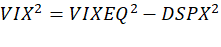• is also a time-series variable: the cap-weighted average variance of the index constituents. You can measure it using trailing daily or monthly returns of each constituent and then combining the 500 variances into one average.
• is a cross-sectional variable: the cap-weighted dispersion of constituent returns. You can measure it using the cross-sectional variance of the 500 constituent returns for a single calendar day or single calendar month. I’ve previously discussed realized monthly dispersion.

These concepts can be applied as backward-looking statistical descriptions of a particular historical sample period, or as forward-looking forecasts of what will happen in the future. We can also look at options markets and infer market expectations. Each of these three concepts has an option-implied index calculated by the Cboe: VIX for market volatility, VIXEQ for individual stock volatility, and DSPX for dispersion.[3]

The equation then becomes:

  (2)

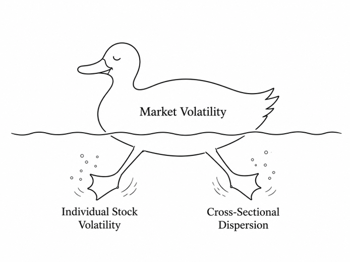
Today’s stock market is often compared to a duck that seems calm above the water but that underneath is paddling madly. It’s a fair description. Figure 1 shows Crazy Legs, the Market Mallard. Its left leg, individual stock volatility, is currently pushing market volatility up. But its right leg, cross-sectional dispersion, is currently pushing market volatility down. Above the surface, Crazy Legs looks calm, but below, its two legs are gyrating wildly in opposite directions.

Figure 1: Crazy Legs, the Market Mallard

Source: Acadian.

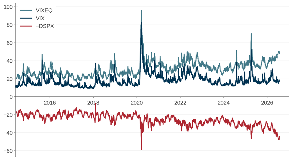
Figure 2 shows the history of the three options-based measures since June 2014 (the start date for VIXEQ and DSPX). The middle line, VIX, is currently around its average level. VIX is pushed up by the top line, VIXEQ, but pushed down by the bottom line, negative DSPX. VIXEQ is currently above the 97^th percentile of its historical distribution, while DSPX is above the 99^th percentile of its distribution.

Figure 2: Implied volatilities and implied dispersion

Source: Acadian based on data from Cboe. For illustrative purposes only.

We can compare today’s market with periods of turmoil such as March 2020 (COVID) and April 2025 (tariff announcements). In these periods, dispersion and individual stock volatility both went up, but individual volatility went up more, resulting in higher market volatility. In contrast, today the rise in individual stock volatility is being offset by the rise in dispersion.

Another way to express the relationship between market volatility and individual stock volatility is using average pairwise correlation. The Cboe also calculates an index of implied correlation, COR1M. Mathematically, there are various identities relating volatilities, dispersion, and correlations. One implication is: [4]

COR1M ≈   (3) 

With VIX fairly calm and VIXEQ sky-high, you immediately know that implied correlation must be low. COR1M is currently around 8%, far below its average level of 37% since 2006 and in the bottom 1% of its historical distribution.

Correlations rise towards one in times of crisis. COR1M hit 97% in October 2008 (the GFC), 96% in November 2011 (Eurozone crisis), and 87% in March 2020 (COVID). Today, we have the opposite situation, with correlations falling towards zero.

Why do we see high dispersion and low correlation? The rational explanation is that AI-related information about corporate fundamentals is impacting different firms differently.[5] Thirukkonda and Roemer (2026) discuss evidence that earnings news has been especially impactful in 2026.

The sentiment-based explanation is that AI mania is causing some stocks to become overvalued and other stocks to become undervalued, with this process generating return dispersion as prices deviate from fundamental value. Campbell, Lettau, Malkiel, and Xu (2023) explore various explanations for changes in dispersion over time and write that:

Investor sentiment can also affect idiosyncratic volatility, particularly over shorter holding periods. Consistent with this, periods of high idiosyncratic volatility often begin during periods of elevated stock prices and intense retail trading activity. During these periods, there is often evidence of extreme optimism and speculation among stock market participants, and idiosyncratic volatility remains high during the inevitable corrections that follow.

One explanation that certainly does not fly is the claim that passive investing is currently distorting prices. If flows in and out of index funds moved stock prices, you’d expect high correlation and low dispersion, which is the opposite of what we see today. Today’s bottom-up, asynchronous market is the polar opposite of a top-down, synchronous market driven by passive flows.

Is it a good thing to have modest market volatility along with high dispersion? If you’re holding the whole index, high dispersion means that maybe you don’t care about the crazy stock-level volatility because it is all cancelling out; less correlated markets are safer markets. The rewards of diversification are greater when dispersion is high and correlation is low.

On the other hand, high dispersion and low correlation have historically been followed by low market returns. As I’ve previously discussed, realized dispersion peaked in December 1999, close to the top of the market. Pollet and Wilson (2010) examine the predictive power of realized correlations and show that times of low correlation are times when subsequent market returns are disappointing.

If you’re holding the index, you’re sitting on top of Crazy Legs, and so far in 2026 you’ve gotten a relatively smooth ride. But if your portfolio deviates from market weights, you’re down in the roiling waters below, a place of great opportunity and great risk. So far, Crazy Legs shows no sign of tiring.

 

---

Endnotes

[1] References to this and other companies should not be interpreted as recommendations to buy or sell specific securities. Acadian and/or the author of this post may hold positions in one or more securities associated with these companies.

[2] Versions of this equation appear in Campbell, Lettau, Malkiel, and Xu (2001), Dew-Becker and Giglio (2023), and in the methodology of the Cboe S&P 500 Dispersion Index.

[3] While option prices also reflect hedging demand, the main determinants of these indices are expectations about future volatility as opposed to risk premia.

[4] This analysis has limitations. Equation (2) is an identity used by Cboe to define DSPX, but it combines mismatched inputs since VIX is based on index options representing all 500 firms while VIXEQ uses only a subset of constituents with liquid options. Equation (3) is an approximation for multiple reasons, including the fact that COR1M uses an even smaller subset of 50 stocks.

[5] Dew-Becker and Giglio (2023) and Morck, Yeung, and Yu (2013) discuss information-based interpretations of dispersion and correlation.

References

Campbell, John Y., Martin Lettau, Burton G. Malkiel, and Yexiao Xu. “Have individual stocks become more volatile? An empirical exploration of idiosyncratic risk.” Journal of Finance 56, no. 1 (2001): 1-43.

Campbell, John Y., Martin Lettau, Burton G. Malkiel, and Yexiao Xu. "Idiosyncratic equity risk two decades later." Critical Finance Review 12, nos. 1–4 (2023): 203–223.

Dew-Becker, Ian, and Stefano Giglio. "Cross-sectional uncertainty and the business cycle: Evidence from 40 years of options data." American Economic Journal: Macroeconomics 15, no. 2 (2023): 65-96.

Morck, Randall, Bernard Yeung, and Wayne Yu. "R² and the Economy." Annual Review of Financial Economics 5, no. 1 (2013): 143-166.

Pollet, Joshua M., and Mungo Wilson. "Average correlation and stock market returns." Journal of Financial Economics 96, no. 3 (2010): 364-380.

Thirukkonda, Ram, and Mark Roemer. “Follow the earnings.” Acadian, July 2026.