
Low-Volatility Investing: Welcoming the Elephant into the Room
Key Takeaways
- The recent disappointing performance of developed market (DM) low-volatility equity strategies has led some asset owners to question the premise of low-risk investing. But we do not believe that the mispricing of equity risk, one of the most robustly documented and conceptually well-grounded market “anomalies,” has suddenly corrected.
- Instead, evaluation of the characteristics of DM low-volatility underperformance, and the market environment that has produced it, points to a solid outlook for low-risk investments.
- Investors would be wise to maintain low-volatility allocations in an investing climate that has been marked by evident speculative pressures.
Table of contents
Over the past few years, low-volatility developed market (DM) equity portfolios have materially underperformed their cap-weighted benchmarks. They experienced significant market-relative drawdowns as stocks surged in 2020-2021 and again in 2023. In the U.S., low-beta equities have produced some of their poorest active returns in at least 60 years.
This recent performance has led some understandably disappointed asset owners to question whether the premise of low-volatility investing has become outmoded. If that were true, then it would signal that one of the most enduring “anomalies” in financial markets, the mispricing of risk within the cross-section of equities, has dissipated. We do not believe that this is the case.
In this paper, we reassess low-risk equity investing. First, we inspect recent low-volatility performance and find nuances that suggest confidence in the outlook. Second, based on examination of high- and low-beta valuations, we caution that investors would be unwise to abandon low-risk DM equity allocations in a market environment that has been rife with speculation. Finally, we demonstrate that the case for a low-volatility allocation is consistent with a wide range of views about prospects for large-cap high-beta stocks; it does not hinge on a view that they are overpriced.
Low-Volatility Performance: Nuances Support a Confident Outlook
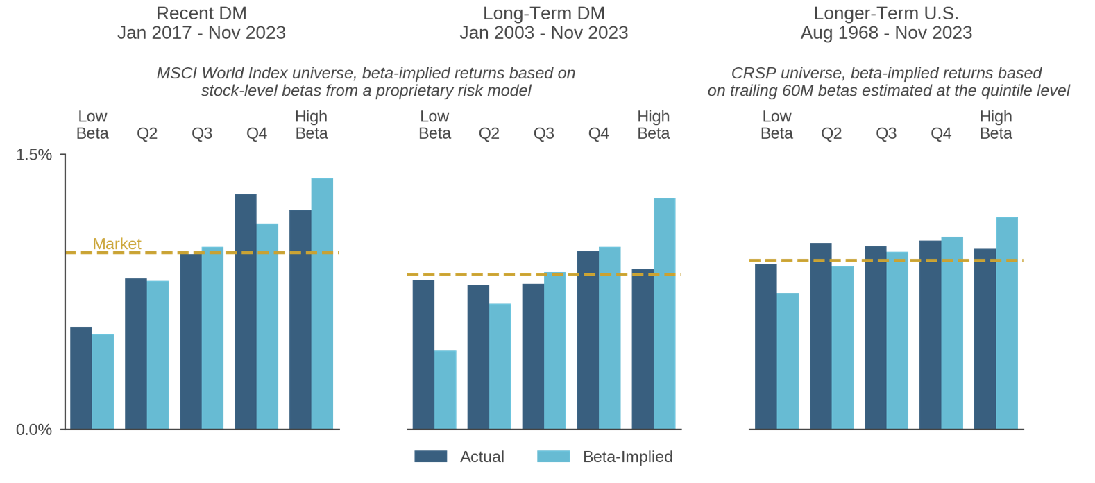
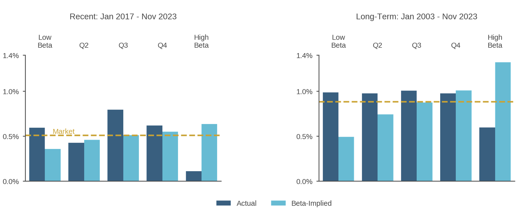
Since 2017, low-beta stocks have underperformed cap-weighted DM equities. Based on the Capital Asset Pricing Model (CAPM), this is exactly what we would expect in a rising market. The left panel of Figure 1 shows that over the cross-section of DM equities, in fact, average returns have roughly corresponded to predictions based on ex ante CAPM betas. Although this relationship is predicted by theory, it is empirically anomalous. The long-term historical regularity is that risk has been mispriced within the equity market: on average, low-beta stocks materially outperform expectations based on their ex ante market exposures, while high-beta stocks materially underperform them. The middle panel of the figure demonstrates the long-term pattern in DM, showing that over the past 20 years there has been little ex post relationship between stock returns and (ex ante) market betas. The right panel extends the evidence back over more than 50 years for the U.S.
Figure 1: The (Mis)Pricing of Risk in DM Equities
Average monthly returns by beta quintile
In summary, the mispricing of risk within equities is a robustly documented phenomenon.1 For nearly 20 years, it has provided the premise of systematic low-volatility investing, i.e., the construction of equity portfolios intended to generate market-like returns with lower volatility and smaller drawdowns.
But the apparent disappearance of the risk mispricing in developed markets over the past few years is leading asset owners and consultants to question this premise. To conclude that it is no longer valid, however, would imply either: 1) the correction of deeply rooted psychological biases that have given rise to the mispricing of equity risk, including investors’ preference for high-risk stocks (e.g., lottery tickets) and overconfidence in assessing valuations, or/and 2) the erosion of limits to arbitrage that have protected the mispricing, including the ubiquity of cap-weighted benchmarks in assessing manager performance.2 We don’t believe that either is the case.
In fact, a close examination of the characteristics of DM low-volatility underperformance reveals several pieces of evidence that lend confidence to the outlook, as we outline below:
#1: DM Low-Volatility Underperformance Reflects a Narrow Phenomenon
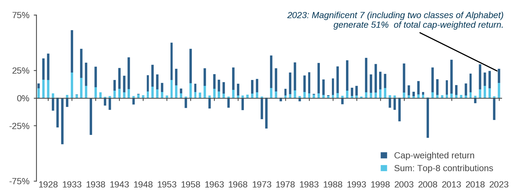
First, welcoming the elephant into the room, low-beta underperformance in DM since 2017 is largely a manifestation of the dramatic run-up in a limited set of high-beta stocks, specifically U.S. tech-oriented bellwethers and most prominently the “Magnificent 7.”3 Figure 2 confirms conventional wisdom that the drivers of benchmark index returns have recently become historically concentrated. The fraction of U.S. cap-weighted performance attributable to a small number of stocks (set at 8 issues in this exhibit to reflect the influence of the Magnificent 7, which contains two classes of Alphabet) has become unusually high and was, in 2023, unprecedented relative to a near century-long history.
Figure 2: U.S. Cap-Weighted Equity Returns and Sum of the Top-Eight Stock Contributions to Them
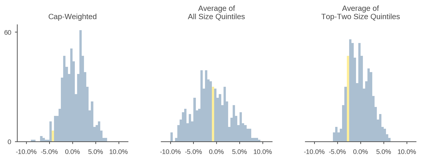
Diverse allocations and active strategies have underperformed MSCI World and other cap-weighted DM benchmarks that have benefitted from material exposure to this narrow group of large-cap stocks; it is hardly a concern unique to DM defensive equities.4 Nevertheless, within the context of low-volatility investing, Figure 3 illuminates the large impact that the narrow sources of cap-weighted returns have had on relative performance. For U.S. low-risk stocks, the charts compare low-beta quintile stock performance to alternative equity benchmarks that modulate the influence of mega caps. While the lowest-beta quintile (cap weighted) has indeed materially underperformed the cap-weighted market since 2017 by 4.5% per annum, it has only underperformed a portfolio that equally weights all size quintiles by 0.5% p.a. and a portfolio that averages the two largest size quintiles by 2.6% p.a. Moreover, while the cap-weighted-relative performance of the low-beta quintile has been truly a left-tail outcome over a 60-year history, its performance relative to the two alternative benchmarks has been unexceptional (57th and 18th percentiles, respectively).
Figure 3: U.S. Low-Beta Performance Since 2017 in Historical Context—Versus Indicated Benchmark
Annualized active return over rolling 84-month windows from 1963-2023; gold bar indicates bin holding the final observation, from 2017-2023
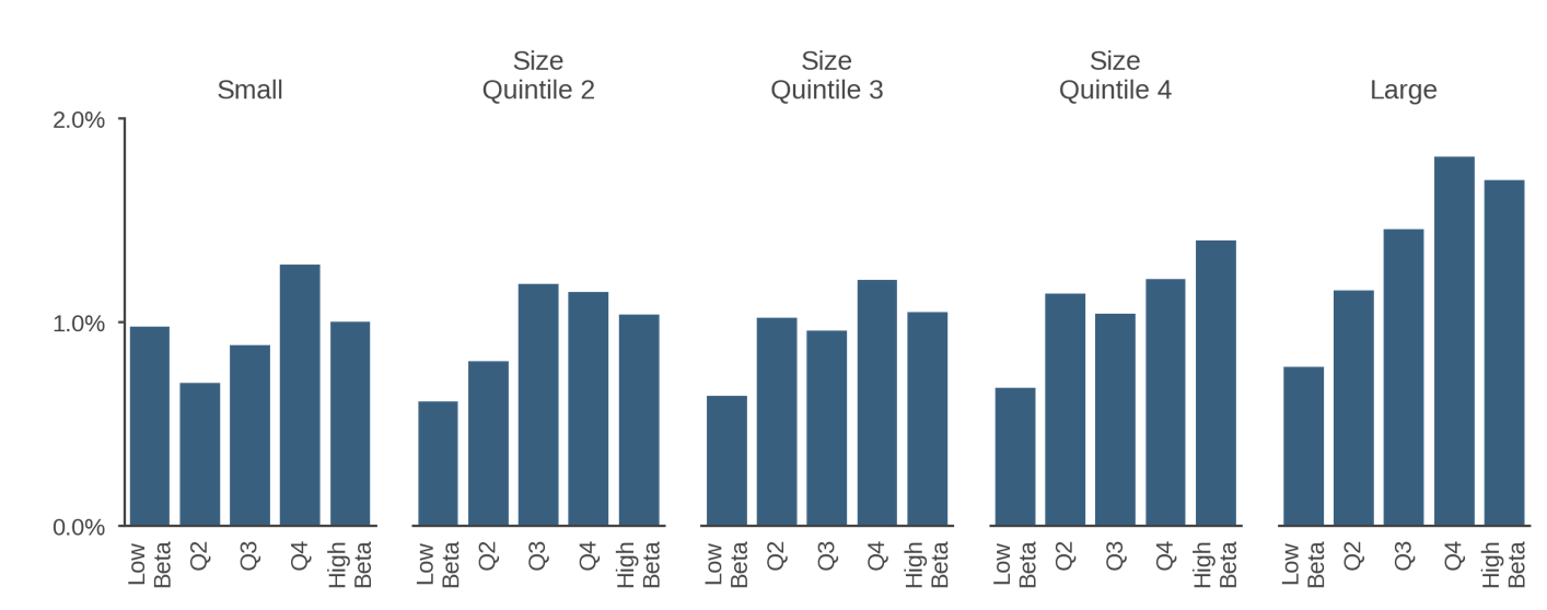
Drilling deeper into these results highlights an additional clue that the premise of low-volatility investing remains sound. Figure 4 shows that in smaller-cap U.S. stocks there has been a weak relationship between beta and returns since 2017.5
Figure 4: Risk Mispricing–Still Evident in U.S. Small-Cap Stocks
Average monthly returns by beta quintile within size quintiles, 2017 – November 2023
#2: Low-Volatility Equities Have Still Provided Downside Protection
While the exceptional run-up in DM high-beta stocks has driven the underperformance of their low-beta complements, when markets have fallen, low-volatility portfolios have continued to provide material relative downside protection. The 2022 selloff provides the salient example. Figure 5 shows that as the MSCI World Index benchmark tumbled more than 20%, the MSCI World Minimum Volatility Index absorbed only 60-75% of the drawdown, depending on the date of measurement.
Figure 5: Drawdown Protection Maintained
2022 MSCI World and MSCI World Minimum Volatility Index performance
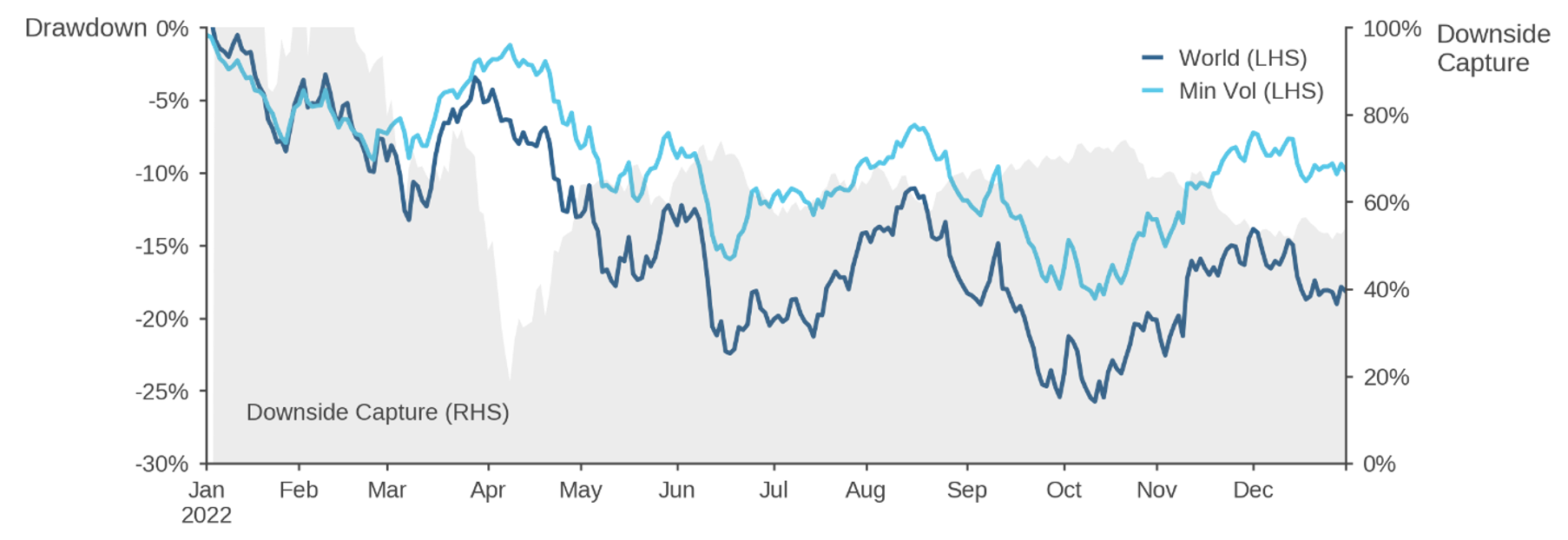
Although low volatility’s downside protection did not manifest to the same degree during the 2020 COVID selloff, we view that episode as an exception that is unlikely to be repeated. The COVID drawdown was unusually brief relative to its severity. As we have discussed in depth in prior research, low beta’s downside protection never had a chance to materialize before it was overwhelmed by the speculatively charged rally that began less than a month after the market initially plunged.6
Looking forward, we do not expect the peculiar circumstances of COVID to become the norm. Rather, we believe that low-beta stocks will continue to outperform during major drawdowns, much as was the case during 2022.
#3: Risk Is Still Being Mispriced in Emerging Markets
Even as low-risk stocks have underperformed in DM, the mispricing of risk has persisted in emerging markets (EM). Figure 6 shows that EM low-risk stocks have kept pace with the cap-weighted benchmark since 2017, while EM high-risk stocks have dramatically underperformed their betas. Broadly speaking, we see no relationship between betas and returns over the EM cross-section in recent years (or over the long term).
Figure 6: Persistence of the Risk Mispricing in EM Equities
Average monthly returns by beta quintile for stocks in MSCI EM Index
We attribute the recent EM-DM low-beta performance discrepancy to a divergence in speculative sentiment across the two market segments. Through late 2020, EM resembled the U.S. in experiencing a speculative run-up in large-cap tech stocks. Since then, however, growth-oriented sentiment in EM has been tempered by the flare-up in U.S.-China geopolitical tensions and China’s economic weakness. Moreover, unlike in 2018-20, when offshore Chinese tech giants enjoyed multiple expansion in a climate of perceived regulatory permissiveness, EM investors have since grown wary of the threat of additional Chinese regulatory pressure, which has helped to keep a lid on valuations.7 As a result, both low-beta stocks (and value signals) fared better in EM than in DM during 2023. The EM experience serves as a cautionary tale that realizations of rosy projections for mega-cap DM growth stocks are not inevitable.
Low-Beta Stocks: Valuation-Based Perspective
Examination of the investing climate that has caused the underperformance of DM low-volatility strategies also lends confidence to their outlook. The run-up in high-beta DM stocks has occurred in a speculatively charged market environment, a historically unusual set of circumstances that we do not expect to persist over the long run.
We documented the emergence of speculation in growthy assets in 2019 and 2022 research on value investing. We showed that in 2017 investors began to aggressively extrapolate the post-GFC earnings increases of large-cap growth stocks, which enjoyed a historically unprecedented run of relative price-to-cash-earnings-multiple expansion as a result.8
Figure 7 reveals how this environment affected low volatility’s market-relative performance in DM. The chart decomposes MSCI World Minimum Volatility and MSCI World Index returns into contributions from changes in 12-month forward earnings, price-to-forward-earnings multiple expansion/compression, and dividends.9 The left panel shows a long-term resemblance: on average, low-volatility and cap-weighted index returns have been similar in composition as well as in magnitude. But since 2017, the decompositions diverge. For the Minimum Volatility Index, rising forward earnings have continued to fuel returns, but forward multiples have compressed, dragging on performance. For MSCI World, in contrast, returns have benefited to a historically unusual extent from forward multiple expansion on top of rising earnings expectations.
Figure 7: Return Decompositions—MSCI World and MSCI World Minimum Volatility Indexes
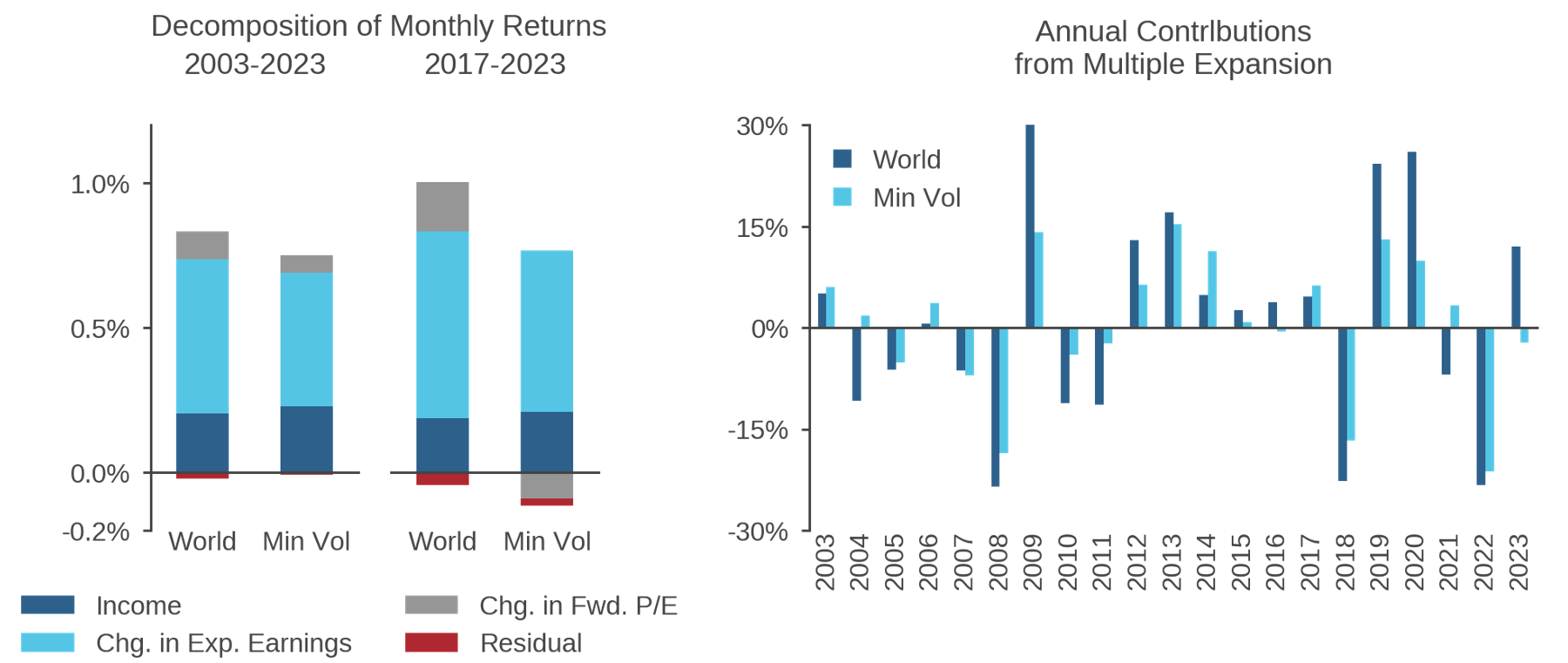
The right panel adds detail, showing how contributions from multiple change have evolved over time. For three of the past five years, MSCI World returns experienced a far greater boost from multiple expansion than the MSCI Minimum Volatility Index, including during the 2020 post-COVID rebound and the 2023 rally.
Inspecting current valuation levels, high-beta forward-earnings multiples look historically unusual. The left panel of Figure 8 shows that in the U.S. high-beta forward P/Es have lingered in a range that is unfamiliar since the TMT bubble. While high-beta valuations cheapened during the 2022 selloff, they dropped less than for the market as a whole. By inference, although high-beta stock prices fell considerably in absolute terms, they dropped less than for other stocks relative to near-term earnings expectations. Moreover, in 2023, high-beta forward P/Es rebounded towards post-COVID highs. Overall, this trajectory suggests that speculative sentiment for high-beta stocks remains strong. In contrast to the historically elevated high-beta valuations, forward P/Es of U.S. low-volatility stocks look unremarkable.
Figure 8: High-Beta Valuations in Context
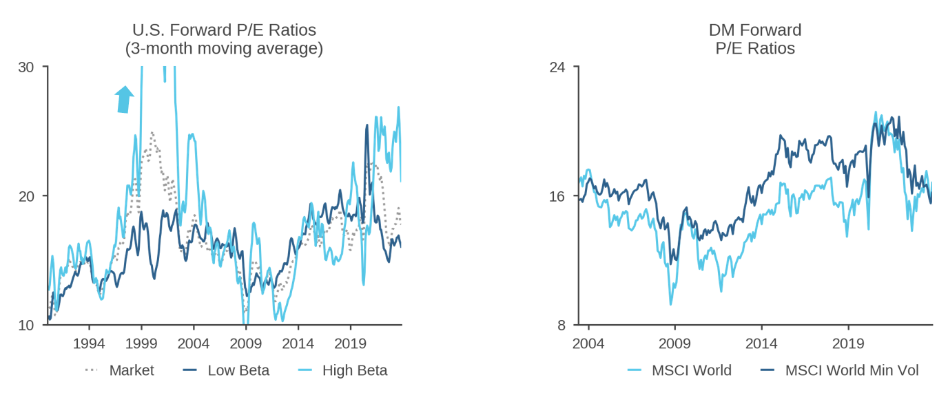
Expanding the view to all of DM, the right panel of Figure 8 shows an interesting shift in MSCI World Minimum Volatility versus MSCI World Index valuations. While for many years the low-volatility index traded at a modest premium to the broader market, consistent with investors paying a premium for stocks with less risky earnings streams, the gap has diminished in recent years. Since COVID, the cap-weighted index has traded in-line with or even at a small premium to the low-volatility index, suggestive of a divergence in market expectations for earnings growth of high- versus low-beta stocks.
In assessing valuations, the salient question for investors is, in essence, whether this time is different. Are the elevated forward valuations that the market is assigning high-beta stocks, and, in particular, a few mega-cap tech-oriented growth stocks, justified?
Providing a definitive answer is beyond the scope of this discussion. We would emphasize, however, that the concern is not whether the Magnificent 7 and other richly priced high-beta companies can continue to generate solid earnings growth, but the degree to which the market is already pricing in that potential. In other words, we can be excited about fundamental prospects for these companies but still conclude that their market prices are too high.
Indeed, there is evidence of speculative froth in recent years. The Baker-Wurgler sentiment index provides a quantification. As shown in Figure 9, market exuberance in the post-COVID environment reached levels rarely seen historically and not since the TMT bubble.10 Amusing corroboration comes from instances of “ticker confusion” on the part of investors so eager to chase meme stocks, like Meta and Zoom, that they did not bother to confirm that they were trading the correct issues. Furniture-maker Ethan Allen even changed its ticker to avoid confusion with a cryptocurrency.
Figure 9: Sentiment and Low-Volatility Returns
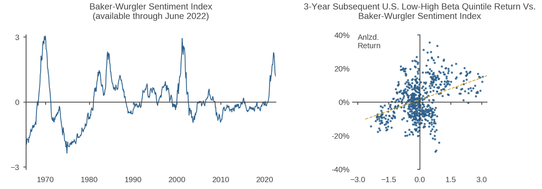
In our view, therefore, investors would be unwise to load-up on a narrow “one-factor bet” on growthy assets in an environment rife with speculative activity. The sidebar, This time is different!?!, recalls dashed expectations in past speculative episodes that bear similarity to present circumstances. Moreover, a mountain of empirical evidence indicates that investors are prone to rationalize overextrapolation of past earnings growth, and surges in sentiment are likely to trigger overvaluation in stocks whose valuations are more subjective, including high-beta stocks.11 In fact, the right panel of Figure 9 offers casual evidence of a link between elevated sentiment and low-beta stock returns, showing that when the Baker-Wurgler sentiment index has been high, stocks in the lowest-beta quintile have subsequently outperformed those in the highest-beta quintile.12
In summary, we believe that it would be a mistake for investors to abandon low-volatility investing in the current environment, and we would encourage asset owners to maintain diversity in the drivers of portfolio performance rather than relying solely on growthy strategies.
Low-Volatility Allocations: Consistent with a "New Normal”
Maintenance of a low-volatility allocation does not have to be predicated on a view that high-beta DM stocks are overpriced. Conceptually, even if their historically rich valuations turn out to be consistent with future fundamental growth, one vision of a “new normal,” then we would still expect the risk mispricing to manifest once more and DM low-volatility performance to improve materially. In the context of the returns decomposition in Figure 7, if the tailwind from (relative) multiple expansion that DM high-beta stocks have enjoyed in recent years subsides, then we would expect an improved outlook for low-volatility strategies. On this basis, therefore, we believe that low-volatility allocations make sense for a wide range of investors—those who are not highly confident that large-cap growthy technology stocks are still undervalued.
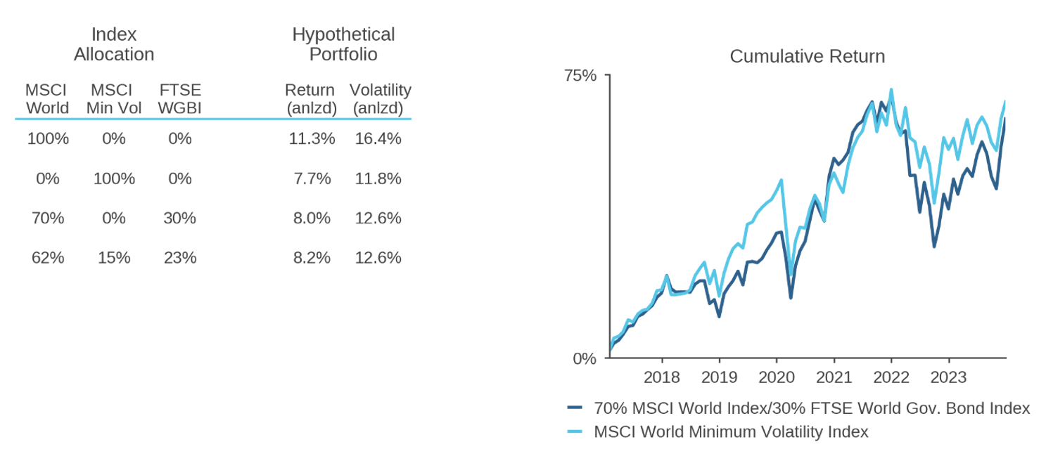
We can reinforce low-volatility’s continued appeal through two hypothetical allocation exercises. The first, highlights that despite the benchmark-relative underperformance of DM low volatility from 2017-2023, investors would still have benefited from adding it to traditional cap-weighted-equity/fixed-income portfolios.
Figure 10 shows that relative to a hypothetical 70% MSCI World/30% FTSE World Government Bond Index (WGBI) mix, for instance, funding a 15% allocation to the MSCI Minimum World Volatility Index by reducing both cap-weighted-equity and bond holdings would have produced superior returns at the same level of volatility. The right chart illuminates the source of the improved performance, showing that the Minimum Volatility Index outperformed a 60/40 MSCI World/FTSE WGBI blend, which would have produced roughly the same level of volatility. Intuitively put, this first exercise highlights that despite low volatility’s cap-weighted underperformance from 2017-2023, it still held appeal for asset owners looking to increase their overall equity exposure.
Figure 10: The Benefit of Adding Low Volatility to a Hypothetical Equity/Fixed Income Portfolio
Based on MSCI and FTSE index return data from 2017-2023
Further reinforcement of the current appeal of low volatility comes from an extension of research by Baker, Taliaferro, and Burnham.13 In a 2017 Financial Analysts Journal article, the authors use a mean-variance-based allocation framework, calibrated to long-term U.S. data, to demonstrate the optimality of holding low-risk equities as part of a broader set of active portfolio exposures. The crux of their finding is that low-risk allocations are additive to a variety of other historically durable equity and fixed income return premia. In other words, the other premia do not subsume the benefits of low-risk investments.14
Figure 11 displays results of a similar exercise that illustrates how the optimal allocation to low volatility would vary depending on an investor’s views about low-volatility and growth stocks.15 Specifically, we optimize allocations among hypothetical value, momentum, quality, and size factors alongside low volatility and growth. Calibrating the exercise using alphas for all six factors and covariances estimated over the full sample from September 2000 – December 2023 produces a baseline result that echoes Baker, Taliaferro, and Burnham’s findings. This outcome, represented by the blue dot on the surface of the chart, shows a substantial optimal low-volatility holding if we use long-term observed performance to ground our expectations for the alphas of all factors.16
Figure 11: Hypothetical Optimal DM Min Vol Allocation as a Function of Min Vol and Growth Expected Alphas
Sharpe Ratio maximized across combinations of equity factor portfolios that have been market neutralized versus MSCI World; based on data from Sep 2000 – Dec 2023
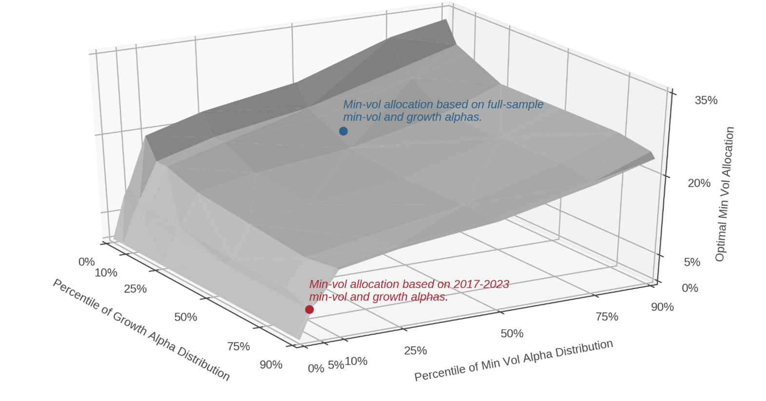
What is of greater interest to this discussion, however, is that material low-volatility allocations are consistent with a wide range of historically observed low-volatility and growth alphas. This is reflected in the flatness of the three-dimensional surface for low-volatility alphas roughly that exceed the 10th percentile of their historical distribution, even for expected growth alphas that are unusually high by historical standards. The red dot, in particular, identifies the hypothetical circumstance where we set ex post alphas for low volatility and growth at values observed from 2017 to 2023, roughly 5th and 90th percentile outcomes, respectively.17 Even with expectations guided by these unusual circumstances, it is still optimal to maintain a positive low-volatility position.
Sidebar: “This time is different!?!”The historically strong performance of large high-beta stocks that has propelled cap-weighted indexes undoubtedly has roots in economic substance. As these stocks have become more expensive, many observers have argued that their valuations are, nevertheless, well justified: “… too many analysts spend too much time worrying about these multiples and not enough time examining the uniqueness of a company… We’re talking about companies where the ability to create and innovate is of a more permanent nature… Go with the best…”18 “The new methods are not based on price-to-book or dividends. They are based on product development, technology promise, … intellectual capital. We have no absolute price-earnings-multiple for a stock… You have to be open about it… Part of our portfolios develop almost like a venture capital fund… We can’t really measure adequately by our normal tools…”19 The buying has come amid a growing consensus that [going forward] the worst that can go wrong… is that stock prices will rise less rapidly than normal… Prices might rise, but at a slower rate than profits, so the price/earnings multiple would drop…20 “By far, the most striking fact… is the degree of unanimity among the people who know the market that it is not irrational, or… even much overvalued. ‘My preliminary guess is that [it] has moved from being a cheap market to just about right…’”21 But these rationalizations are not referring to valuations of the Magnificent 7 or modern AI companies. They are all from historic periods of market overextrapolation: the first from the “Nifty-Fifty” era in 1972, the second from the dotcom bubble in January 2000, and the last two from the twilight of the great Japanese asset price bubble of the 1980s. In each of these cases, investors found convincing explanations for sustained run-ups in concentrated groups of stocks. Like the strong performance of technology stocks over the past several years, the dotcom and Japanese bubbles dramatically altered the composition of cap-weighted market benchmarks and, along the way, distorted metrics of investing success. The “Nifty Fifty” differed in character from the other two episodes and has a special relevance. The Nifty-Fifty moniker references a somewhat nebulous group of 20-50 prominent U.S. growth stocks, including IBM, MMM, Xerox, McDonalds, Digital Equipment, Polaroid, Kodak, Disney, and Avon, that trust departments of leading banks prized during the early 1970s.22 In an era of wobbly sentiment after the “go-go” bull market of the 1960s had faded amid the inflationary pressures and instability associated with the Vietnam War, these stocks were prized for consistent track records of earnings growth and dividend increases as well as their substantial capitalizations—in contemporary terms, because they were quintessential large-cap, high-quality growth stocks. Lofty price-earnings ratios were one of their defining characteristics, and these companies were viewed as being worthy of them. For a time, that view seemed well justified. As one reporter wrote in 1974, “The astonishing thing was that most of the so-called nifty-fifty stocks maintained their strength through four of the worst years in modern market history.”23 But the Nifty Fifty eventually suffered during the bear market of the 1970s. And while there has been disagreement as to whether the Nifty Fifty were overvalued as a whole in 1972, there is little question that the most elevated P/E ratios among the Nifty Fifty turned out to be unwarranted.24 The point of examining these past episodes is not to forecast that the Magnificent 7 and other high-beta stocks are due for some kind of imminent reckoning. Rather, it is a reminder that investors tend to overextrapolate performance and to find convincing rationalizations for doing so. Things might turn out to be different this time, and lofty market valuations driven by relatively narrow sources of performance might turn out to be justified. But investors would be unwise to reflexively presume that they are, and their portfolios should reflect the probabilities of other outcomes. |
In summary, intuition and hypothetical allocation exercises underscore that most active investors should maintain material low-volatility exposure even if they are bullish on growth stocks. To warrant zeroing out the low-volatility allocation would take a high-conviction view that those stocks are likely to generate historically poor performance going forward. The relevant question for most investors, then, is not whether they should hold low-volatility allocations, but how those positions should be sized.
Conclusion
Without exaggeration, it would be a stunning development if equity risk were no longer mispriced in the cross section. That the CAPM does not actually hold, in practice, is one of the best-documented and conceptually well-grounded “anomalies” in modern finance. Despite the recent underperformance of low-risk investments in developed markets, we do not believe that the mispricing of equity risk has dissipated. Instead, evaluation of the characteristics and drivers of recent returns, and the market environment that has produced them, suggest that prospects for low-risk investing remain solid. As such, we believe that investors would be prudent to maintain low-volatility allocations, especially in a market environment where there has been evident speculative pressure.
Appendix: Specifications of the Hypothetical Allocation Analysis in Figure 11
| Full sample period: | September 2000 – December 2023. |
| Candidate strategies: | Hypothetical DM factor portfolios generated from returns of MSCI World Minimum Volatility, Growth, Value, Momentum, Small Cap, and Quality Indexes. Contributions to returns from the MSCI World Index are removed via in-sample estimation of each factor portfolio’s (univariate) beta to the MSCI World Index. |
| Expected alphas: | For strategies other than minimum volatility and growth, expected alphas are set equal to full sample alphas estimated relative to MSCI World Index. For minimum volatility and growth, alphas are varied between the minimum and 90th percentiles of historical alphas over rolling 84-month periods over the full sample period. |
| Expected risk: | Set at observed volatilities of and correlations between returns of candidate strategies (residualized versus MSCI World Index) calculated over the full sample period. |
| Portfolio construction: | Sharpe Ratio maximization with bounds on individual strategy allocations between 0% and 33.33%. This restriction implies that at least 3 strategies will be held in the optimal portfolio. The strategies have different historical volatilities, which implies that equivalent percentage allocations make different contributions to risk. Because the purpose of the exercise is to illustrate a high-level conclusion rather than to recommend any specific allocation, we make no adjustment to put candidate strategies on an equal risk footing. |
Endnotes
- The risk mispricing has been documented not just over time but also across geographies and even in other asset classes. For evidence of mispricing of risk in cryptocurrencies, for example, see Quick Take: Fortune Favors the… Boring?, Acadian, February 2022.
- See, for example, Malcolm Baker, Brendan Bradley, and Jeffrey Wurgler, “Benchmarks as Limits to Arbitrage: Understanding the Low-Volatility Anomaly.” Financial Analysts Journal 67, no. 1 (January/February 2011) and Malcolm Baker, Brendan Bradley, and Ryan Taliaferro, “The Low-Risk Anomaly: Decomposition into Micro and Macro Effects.” Financial Analysts Journal 70, no. 2 (March/April 2014).
- Nvidia, Tesla, Meta, Apple, Amazon, Microsoft, and Alphabet. References to these and other companies in this write up should not be construed as recommendations to buy or sell specific securities.
- For example, in 2020 research we pointed out that large-cap U.S. growth stocks had, over the prior 10 years, outperformed a broad swath of country equity indexes, sovereign bonds, currencies, and commodities. See Re-examining Diversification 20/20 Perspective, Acadian, June 2020.
- Ken French forms size quintiles based on NYSE breakpoints.
- All stocks, even those with low ex ante betas, typically suffer severe losses during the initial phases of sharp selloffs as fear-struck investors indiscriminately sell equities, a phenomenon called “beta compression.” But as bear markets age, low-volatility stocks usually begin to outperform as investors embrace their less-risky fundamentals. Figure 5 illustrates that the typical pattern emerged during 2022. The MSCI World Minimum Volatility Index initially fell in lockstep with MSCI World but provided significant downside protection as the drawdown deepened. During the brief 2020 COVID selloff, this usual pattern had no time to manifest. For detailed discussion, see Managed Volatility in the Pandemic: The One-Year Anniversary, Acadian, March 2021.
- See Quick Take: EM Low Vol Equity as Risk Aversion Returns, Acadian, August 2021.
- For detailed discussion, see Returns to Value: A Nuanced Picture, Acadian, November 2019 and Growth Versus Value: End of an Era?, Acadian, November, 2022.
- In this decomposition, there is also a residual attributable to the interaction between the change in 12M forward earnings estimates and the price-to-forward earnings multiple expansion.
- The chart displays the SENT series from the August 2022 update of the index found at https://pages.stern.nyu.edu/~jwurgler/. This version of the index represents a composite of five measures of risk-seeking activity in equities, including first-day IPO returns, IPO volume, the closed-end fund discount, the equity share of new issues, and the value-weighted dividend premium (relative valuation of dividend payers and non-payers).
- See Malcolm Baker and Jeffrey Wurgler, “Investor Sentiment in the Stock Market.” Journal of Economic Perspectives 21, no. 2 (Spring 2007) 129-151.
- This observation is not intended as evidence that it is profitable to time low-volatility allocations based on sentiment. The Baker-Wurgler sentiment index is not point-in-time. It contains lookahead information, e.g., a full in-sample time series normalization.
- The factors included are low volatility, value, quality, momentum, size, interest rate term, and credit. See Baker, Malcolm, Ryan Taliaferro, and Terry Burnham. “Optimal Tilts: Combining Persistent Characteristic Portfolios.” Financial Analysts Journal 73, no. 4 (Fourth Quarter 2017): 75–89.
- Especially after accounting for transaction costs.
- See the Appendix for details of the analysis.
- In this exercise, the optimal minimum volatility allocation is 19%. This percentage should not be construed as a recommended allocation to any particular low-volatility strategy within any broader portfolio.
- We choose rolling 84-month windows to correspond with the length of the 2017-2023 period.
- Interview with John L. Furth of E. M. Warburg Pincus and co-author of “Shaking the Money Tree” in “Authors Take a Look at Growth Stocks,” The New York Times, June 5, 1972.
- Interview with Richard Driehaus of Driehaus Capital Management in “Steller Year for a Standout Stock Picker,” The Washington Post, January 23, 2000.
- The New York Times, March 7, 1989.
- South China Morning Post, March 12, 1989, quoting Andrew Smithers of SG Warburg.
- See Robert Metz, “Compensating Money Managers,” The New York Times, October 19, 1974.
- Ibid.
- In Jeremy Siegel’s 1998 analysis of the Nifty Fifty, none of the stocks in the top quartile of actual 1972 P/Es lived up to those valuations based on subsequent data through 1998. Compare “1972 Actual P/E” to “Warranted P/E Ratio” in Table 1 of Jeremy Siegel, “Valuing Growth Stocks: Revisiting the Nifty Fifty,” AAII Journal, October 1998. See also Jeff Fesenmaier and Gary Smith, “The Nifty-Fifty Re-Revisited,” The Journal of Investing, Fall 2002, 11(3) 86-90.
Hypothetical
Acadian is providing hypothetical performance information for your review as we believe you have access to resources to independently analyze this information and have the financial expertise to understand the risks and limitations of the presentation of hypothetical performance. Please immediately advise if that is not the case.
Hypothetical performance results have many inherent limitations, some of which are described below. No representation is being made that any account will or is likely to achieve profits or losses similar to those shown. In fact, there are frequently sharp differences between hypothetical performance results and the actual performance results subsequently achieved by any particular trading program.
One of the limitations of hypothetical performance results is that they are generally prepared with the benefit of hindsight. In addition, hypothetical trading does not involve financial risk, and no hypothetical trading record can completely account for the impact of financial risk in actual trading. For example, the ability to withstand losses or to adhere to a particular trading program in spite of trading losses are material points which can also adversely affect actual trading results. There are numerous other factors related to the markets in general or to the implementation of any specific trading program which cannot be fully accounted for in the preparation of hypothetical performance results and all of which can adversely affect actual trading results.
Legal Disclaimer
These materials provided herein may contain material, non-public information within the meaning of the United States Federal Securities Laws with respect to Acadian Asset Management LLC, Acadian Asset Management Inc. and/or their respective subsidiaries and affiliated entities. The recipient of these materials agrees that it will not use any confidential information that may be contained herein to execute or recommend transactions in securities. The recipient further acknowledges that it is aware that United States Federal and State securities laws prohibit any person or entity who has material, non-public information about a publicly-traded company from purchasing or selling securities of such company, or from communicating such information to any other person or entity under circumstances in which it is reasonably foreseeable that such person or entity is likely to sell or purchase such securities.
Acadian provides this material as a general overview of the firm, our processes and our investment capabilities. It has been provided for informational purposes only. It does not constitute or form part of any offer to issue or sell, or any solicitation of any offer to subscribe or to purchase, shares, units or other interests in investments that may be referred to herein and must not be construed as investment or financial product advice. Acadian has not considered any reader's financial situation, objective or needs in providing the relevant information.
The value of investments may fall as well as rise and you may not get back your original investment. Past performance is not necessarily a guide to future performance or returns. Acadian has taken all reasonable care to ensure that the information contained in this material is accurate at the time of its distribution, no representation or warranty, express or implied, is made as to the accuracy, reliability or completeness of such information.
This material contains privileged and confidential information and is intended only for the recipient/s. Any distribution, reproduction or other use of this presentation by recipients is strictly prohibited. If you are not the intended recipient and this presentation has been sent or passed on to you in error, please contact us immediately. Confidentiality and privilege are not lost by this presentation having been sent or passed on to you in error.
Acadian’s quantitative investment process is supported by extensive proprietary computer code. Acadian’s researchers, software developers, and IT teams follow a structured design, development, testing, change control, and review processes during the development of its systems and the implementation within our investment process. These controls and their effectiveness are subject to regular internal reviews, at least annual independent review by our SOC1 auditor. However, despite these extensive controls it is possible that errors may occur in coding and within the investment process, as is the case with any complex software or data-driven model, and no guarantee or warranty can be provided that any quantitative investment model is completely free of errors. Any such errors could have a negative impact on investment results. We have in place control systems and processes which are intended to identify in a timely manner any such errors which would have a material impact on the investment process.
Acadian Asset Management LLC has wholly owned affiliates located in London, Singapore, and Sydney. Pursuant to the terms of service level agreements with each affiliate, employees of Acadian Asset Management LLC may provide certain services on behalf of each affiliate and employees of each affiliate may provide certain administrative services, including marketing and client service, on behalf of Acadian Asset Management LLC.
Acadian Asset Management LLC is registered as an investment adviser with the U.S. Securities and Exchange Commission. Registration of an investment adviser does not imply any level of skill or training.
Acadian Asset Management (Singapore) Pte Ltd, (Registration Number: 199902125D) is licensed by the Monetary Authority of Singapore. It is also registered as an investment adviser with the U.S. Securities and Exchange Commission.
Acadian Asset Management (Australia) Limited (ABN 41 114 200 127) is the holder of Australian financial services license number 291872 ("AFSL"). It is also registered as an investment adviser with the U.S. Securities and Exchange Commission. Under the terms of its AFSL, Acadian Asset Management (Australia) Limited is limited to providing the financial services under its license to wholesale clients only. This marketing material is not to be provided to retail clients.
Acadian Asset Management (UK) Limited is authorized and regulated by the Financial Conduct Authority ('the FCA') and is a limited liability company incorporated in England and Wales with company number 05644066. Acadian Asset Management (UK) Limited will only make this material available to Professional Clients and Eligible Counterparties as defined by the FCA under the Markets in Financial Instruments Directive, or to Qualified Investors in Switzerland as defined in the Collective Investment Schemes Act, as applicable.