Machine Learning in Quant Investing: Revolution or Evolution?

As a society, we’ve become preoccupied with “the rise of machines”; the topic taps into some of the greatest hopes and fears of our digital age. In the financial world, though, the breathless and superficial nature of the broader cultural dialogue around it has clouded understanding as to what actual impact artificial intelligence, machine learning, and the explosion of data will have over the foreseeable future.

In this note, we ground the discussion by laying out our view as to how ML will reshape quantitative investing over the next few years. We contextualize ML approaches relative to traditional methods, considering their salient characteristics, principal advantages, and scope of application as well as challenges to their further integration. To provide a real-world sense of what it means to apply ML in quant investing, we present a  brief case study involving the enhancement of a stock-selection signal. 

In summary, ML significantly expands the analytical toolkit for sophisticated quantitative investors. We believe that it already is generating material additional value and will deliver more. ML has application throughout the investment process, including nonlinear forecasting, revealing structure in complex data, and derivation of quantitative metrics from qualitative information. But the application of ML to investing is more challenging than in many other contexts. As a result, financial domain knowledge and a rigorous and explicit research process will be essential for sustained success. Awareness of these considerations will help asset owners to distinguish true value-add from naive data mining.

ML in Context

Artificial intelligence represents a broad goal: development of machines that make decisions at  least as well as humans. Machine learning is an  approach to achieving that objective: data-driven computer applications that train themselves to complete complex tasks without explicit instruction. (See the Appendix for a primer on three popular machine learning approaches.)

AI and ML concepts and methods are not new, and attempts to apply them to investing date back decades. In the 1990s, for example, numerous academic articles extolled the promise of neural networks to forecast stocks, currencies, and financial events.¹

Today, the intense focus on ML reflects the confluence of several trends. First, many ML methods are computationally intensive, and computing costs have dropped dramatically. Commoditization of cloud computing has made thousands of processors available on-demand. Second, ML algorithms are now freely available in robust and well-documented opensource packages, dramatically lowering cost, time, and knowledge barriers to implementation. Third, the explosion of big data facilitates ML approaches that involve algorithms with hundreds or thousands of parameters to estimate, and that therefore require enormous quantities of data to train. Finally, there have been algorithmic breakthroughs, including in language processing and the development of better behaved and more computationally efficient neural networks.

In the context of quant investing, interest in ML reflects desire for greater modeling flexibility in two broad respects. The first is non-linear prediction. ML algorithms are designed to infer the relationship between data attributes and a variable of interest. In contrast, ubiquitous linear regressions impose an assumption that the form of the relationship is a straight line. Although linear models have endured for a host of good reasons, including simplicity, transparency, robustness, and modest data requirements, in many investing contexts the assumption of linearity is unfounded, and neither theory nor intuition suggests a particular alternative. Examples include forecasting probabilities of market events or economic regime shifts.²

A second motivation for ML is to reveal hidden structure in complex, large data sets. In identifying a company’s peer group, for example, ML algorithms may help to illuminate the economic relationships among hundreds of firms, simultaneously accounting for numerous attributes. ML can also help to expose interactions between predictive variables that may  vary with environmental conditions. ML-based textual analysis can derive quantitative metrics from  qualitative information, sentiment analysis being a prominent example.

ML techniques represent a significant expansion of the quantitative investor’s toolkit, but they’re not qualitatively distinct from traditional statistical methods. Linear regression, for example, can be expressed as a simple neural network. Elements of ML algorithms to identify the most valuable predictive variables and to avoid overfitting have analogues in conventional statistical methods. As a result, trying to identify a meaningful bright-line demarking traditional approaches form ML would be a fruitless exercise. Fortunately, it’s also not important. 

Of great consequence, however, are the implications of easy access to more flexible but also more opaque analytical tools. For quantitative investment managers, it opens new avenues of research that have genuinely exciting potential. Yet their enduringly successful exploitation will demand considerable effort and firm commitment to a disciplined research process. And while ML methods require new skill sets, domain knowledge from finance will remain crucial to beneficial research.

For asset owners, the increased modeling flexibility will exacerbate challenges in manager and strategy selection. Finance is already rife with sloppy data mining, and access to a more expansive toolkit only makes it easier. Further, the opacity of some ML approaches will complicate performance attribution even when such techniques are implemented appropriately. As a “canary in the coal mine” regarding such challenges, the data science literature is already replete with claims of unrealistic market forecasting ability. In this evolving environment, a working knowledge of ML techniques and research best practices will help to protect asset owners. 

An ML Case Study

To demonstrate the application of ML to quant investing, we present a case study in the enhancement of a stock-selection signal. In a 2002 paper, Joseph Piotroski proposed an approach to improve valuation factors for bottom-up stock picking.³ The premise was that conditioning on indicators of a company’s fundamental strength can help to distinguish attractively undervalued stocks from value traps. Today, the general concept of employing quality variables to help identify underpriced fundamentals is well established. Nevertheless, Piotroski’s framework is worth revisiting as an intuitive, real-world setting in which to highlight motivations for applying ML and to elucidate the ML research process.

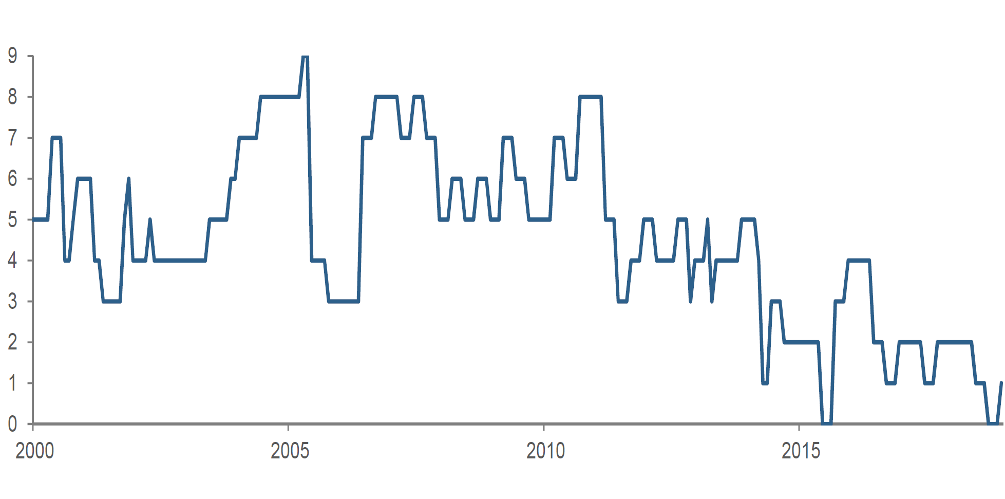
To test his hypothesis, Piotroski formed a composite indicator, which he called the “F-score.” (Figure 1) This was constructed from nine inpidual financial statement metrics chosen to reflect 1) profitability, 2) leverage, liquidity, and source of funding, and 3) operating efficiency. To put the data items on an equal footing so that they could be combined, Piotroski took a sensible and robust approach. For each attribute, he created a binary variable, assigning a 1 if the attribute were positive and 0 if negative. For each stock on each date, he then summed the binary variables to create the baseline F-score signal.⁴ Exemplifying the signal’s intuition, Figure 2 shows that Sears Holdings’ F-score captured a protracted deterioration in the company’s financial strength in the years prior to its bankruptcy.

Figure 1: Creating the "F-score"

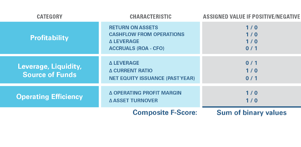
Figure 2: Sears Holdings' F-score

Why ML?

This is an appealing setting in which to apply ML for several reasons. First, we have intuition that the selected financial characteristics may help return forecasting capabilities; this isn’t an uninformed fishing expedition in a low signal-to-noise-ratio environment. Second, although reducing the inpidual financial attributes to binary variables and then summing them is intuitive and transparent, we have no reason to think that it fully exploits their predictive value. Third, there is no theory or intuition to suggest how we should combine the inpidual quality metrics, e.g., whether to accord each equal weight or whether the predictors interact. Fourth, we don’t know what the relationships between F-score components and future returns look like; they may be unequal and/or highly non-linear.

Specifying an ML Approach

To develop and evaluate an ML-based alternative signal, we follow a research process that has three interrelated elements:

• Data preparation: We must decide what data inputs to feed into the machine. This involves: 1) selection of candidate predictive variables (“features”), 2) data preprocessing, i.e., cleaning and integration, and 3) transformations of the raw data, e.g., market or peer group adjustments and normalizations. For this case study, we work with Piotroski’s selected attributes.⁵ Preprocessing includes treatment of missing and outlier predictor values, exclusion of financials, and a filter for tradability. We also market-adjust stock returns.
• Algorithm selection: For this exercise, we choose an approach called “random forest.” In data science circles, this method is considered a solid, general purpose algorithm. It’s relatively easy to implement, generally effective and robust, and reasonably transparent.
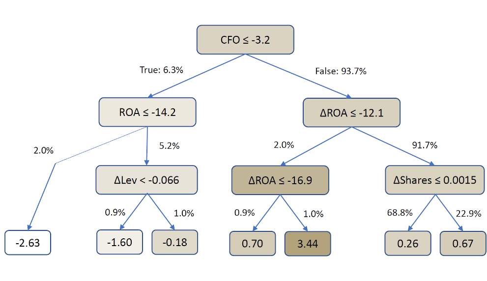
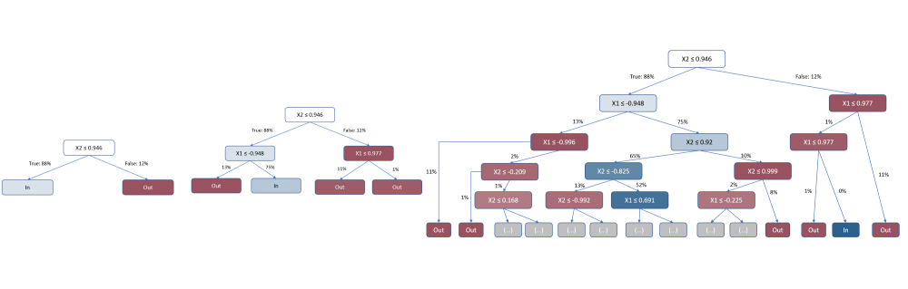
  By way of high-level description, the random forest algorithm is based on generating many “decision trees” fitted to historical data. An inpidual decision tree, an illustrative example of which is shown in Figure 3, represents a sequence of simple forecasting rules each of which, in the case study, relates an inpidual accounting variable to future returns. Specifically, at each decision point in the tree, called a node, the algorithm subpides the training data into two groups of observations based on the value of one attribute. The algorithm selects the attribute on which to split the sample so as to most effectively discriminate between higher and lower future returns in the training sample. Not every variable may appear in a tree; i.e., the algorithm may find that certain attributes don’t have predictive power, and a variable may appear several times, associating its different levels with a range of predicted returns. (See the Appendix for further discussion of decision trees.)
  In a “random forest” implementation, we generate many trees, fitting each one from a random subset of the historical data. The purpose is to reduce the risk of overfitting associated with estimating just a single tree, which might be driven by spurious relationships in the full sample. We generate the final return forecast for new, out-of-sample observations by averaging return forecasts across all the fitted trees. For the case study, we estimated between 300 and 3,000 trees per forest in various candidate implementations.
• Data sample management: Implementing an ML algorithm typically involves subpiding the historical dataset into three segments: 1) a “training” sample to estimate algorithm parameters, 2) a “validation” sample to tune the algorithm and/ or select among several variants, and 3) “out-of-sample” historical data to evaluate the approach.
  For this case study, we used the validation step to choose the maximum number of nodes in the decision tree (tree “depth”) and other criteria to limit the branching process. The purpose of these restrictions is to avoid overfitting and reduce sensitivity to outliers. We trained and validated the random forest algorithm based on data from 2000-2012, and we ran it out-of-sample from 2013-2018. We restricted tree depth to 3 levels.

Figure 3: Sample decision tree

Results

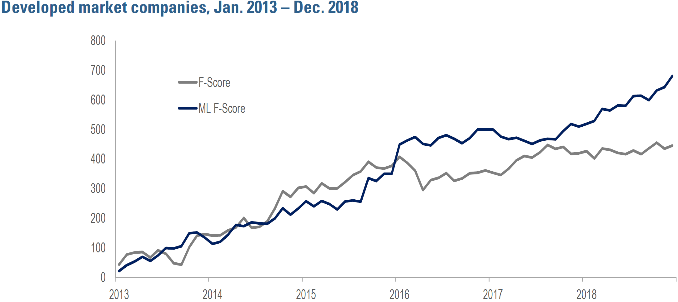
Figure 4 compares the predictive efficacy of the baseline and ML-based F-score signals in a broad universe of developed market stocks from 2013-2018. The table  shows that the ML-based version displays greater  efficacy in predicting stocks’ 1-month-ahead returns, as 
evidenced by a higher slope coefficient (9.4bp/month versus 6.2bp/month). Its predictive ability is highly statistically significant (t-stat of 3.7 versus 2.3 for the baseline version).⁶ 

Figure 4: Efficacy Comparison – baseline F-score vs. ML F-score

Analysis of inpidual trees within the random forest reveals that the forecasts are primarily driven by cash flow from operations followed by the change in return on assets, whereas change in gross margin, current ratio and leverage have limited influence.  This variation contrasts meaningfully with the baseline F-score’s implicit equalweighting scheme across the nine attributes. Interestingly, even though the ML formulation is materially driven by cashflow from operations, its direct correlation is modest.  This likely reflects the non-linear nature of decision trees and, consequently, the random forest itself.  As well, the ML F-score signal has a fairly long workout horizon and high serial correlation, which suggest that it wouldn’t induce excessive turnover.

Opportunities and Challenges

ML’s added flexibility has application throughout the investment process. Motivations for the case study  help to explain why certain contexts make for promising use-cases, and special challenges in applying ML to a market context help to explain why some uses-cases hold less appeal.

Generation of new quant data inputs: ML is already extensively used to create alternative data sets, with language processing of news, filings, and social media among prominent examples. Contemporary applications include sentiment measurement, event detection, and evaluation of qualitative relationships and risks. Inferring context in unstructured, long-form text remains a challenge, and this use-case is helping to drive development of deep learning methods. Data imputation is another area well-suited to ML. Examples in the context of company fundamentals would include detecting errors and estimating missing or late-reported data items. ML techniques may be able to exploit underlying accounting logic or management behaviors that generate subtle, predictable patterns in the data.

Returns forecasting: ML has broad potential in forecasting. Examples include enhancement of technical signals (i.e., signals related to historical patterns in returns), where flexible ML-based prediction can better exploit richness in the data than prior generations of indicators that traded off informational nuance for robustness. As well, ML is already incorporated into sophisticated cross-asset technical signals to help identify subtle linkages among securities.

But history is littered with forgotten academic articles and dead weblinks that chronicle persistently unrealistic expectations among methodologically sophisticated but market-naive data miners. When working in financial markets, ML researchers must recognize that the signal to noise ratio is lower and  the data-generating environment more unstable than  in many other contexts in which such methods are being applied.

Risk forecasting: There is no consensus as to the form of the underlying process driving financial market volatility despite decades of empirical research. Innumerable complex statistical models have been proposed to describe and predict its dynamics, including “jumps” and “regime shifts.” In this context, the gap between past statistical approaches and ML seems particularly indistinct. At the portfolio level, evaluating and forecasting risk depends on capturing the comovement among the component instruments. The task usually involves some form of “dimensional reduction,” i.e., identifying common drivers of returns, a natural context for the application of “unsupervised” learning algorithms.⁷ ML also has application in predicting risk events, a setting that motivates nonlinearity and where training datasets of past events usually are easy to construct.

Factor weighting: Shifting factor exposures as macroeconomic and risk conditions evolve is oft-cited as an area of potential ML benefit. The premise being that flexible analytical approaches may be able to detect market regime shifts and adapt weightings appropriately. This use-case presents challenges, however. Among them, we may not have observed enough relevant historical transitions between states to train data-hungry algorithms, and investors may be particularly uncomfortable with reduced transparency during periods of market stress.

Implementation: ML has achieved comparatively wide use in high frequency trading in part because there is an enormous amount of intraday data that can be used to train execution algorithms. As well, in an era of market fragmentation, optimal choice of venue, method, and timing likely depends on many conditioning factors, including expected volumes and order flow, upcoming events, and sentiment. Optimizing over this large and complex set of inputs is a task well-suited to inductive ML processes.

Best Practices

In identifying promising ML applications, the nature of  the variable being forecasted and availability of historical data emerge as consistent themes. In many investing contexts, the low signal-to-noise ratio and relative scarcity of training data imply that blindly unleashed ML algorithms are prone to overfitting, i.e., picking up on spurious relationships in training data that are of no use in forecasting out-of-sample.

While finance has long been rife with sloppy and abusive data mining, we expect that ML’s flexibility  and opacity will increase its prevalence. For asset  owners this will exacerbate challenges in distinguishing value-added approaches from artifacts of backtesting and slick presentation.

This concern informs a set of best practices to watch for in ML’s application to investing. It should be guided by understanding of a specific problem, and algorithms must be carefully controlled and validated to have out-of-sample efficacy. ML is generally applied for data mining rather than hypothesis testing, i.e., with the objective of maximizing predictive power rather than providing insight. With that frame of reference in mind, the research process outlined in the case study is expressly designed to provide “guardrails” that reduce the risk of overfitting.

Investment expertise will remain crucial to beneficial ML research. Decisions regarding data preparation, algorithm selection, and data sample management are interdependent, and investment domain knowledge informs them. As one example, judicious data preparation reduces the amount of data required for training and validation. Relying on ML to derive a peer-relative transformation likely would require an extremely  flexible and data intensive algorithm and increase the  risk of overfitting. 

Because overfitting is such a prominent concern, overreaction to that risk may lead to underfitting. Techniques designed to reduce fitting noise can result  in losing a signal altogether. While need for transparency should influence the decision to apply ML as well as algorithm selection, concern about complexity and opacity may lead to excessive caution in ML’s application.

While understanding the drivers of algorithm behavior can be a challenge, even in the context of complex ML methods we may nevertheless have means to gain insight. For a decision tree, inspecting early branches reveals which features the algorithm deems most predictively valuable, and, as we demonstrated in the case study, we can derive summary statistics of relative feature importance. For a neural network, the first “hidden layer” of nodes may serve as a feature-identification step, filtering and combining raw inputs into more refined items that are then passed deeper into the system. We may also be able to assess an algorithm’s likely response to circumstances of special interest by feeding it contrived data.

As well, many longstanding research best practices remain applicable to ML contexts. These include comparing an ML-based forecaster’s behavior to simpler, more transparent signals, analyzing whether it loads on known risk factors, and examining whether its serial correlation and workout horizon suggest that it will induce portfolio instability and high turnover. Integration of ML doesn’t necessarily turn the investment process into an impenetrable black box. 

Conclusion: The Outlook

ML is already a part of sophisticated quants’ investing toolkit. It offers valuable modeling flexibility and has application throughout the investment process. We view the integration of ML into investing as an evolution rather than a revolution. The techniques aren’t qualitatively distinct from traditional methods, and we expect that the quantitative investment process will remain recognizable in the foreseeable future, even as the research tools that inform its components evolve. Markets make for an especially challenging environment in which to apply ML, and beneficial ML-based research calls for process discipline and finance domain knowledge. For asset owners, more flexible but more opaque analytical tools  will exacerbate challenges in distinguishing strategies  that add value from data artifact. Working knowledge of ML approaches and ML research best practices offer a valuable defense.

Appendix

ML Methods: A Primer for Investing Practitioners

This Appendix provides insight into three of the most prevalent machine learning approaches, decision trees, support vector machines, and neural networks. We make use of an illustrative “binary classification problem” where the goal is to categorize data observations into two groups. In medicine, problems of this form would include identifying tissue samples as cancerous or noncancerous; in investing, examples would include seeking to predict whether a market index may rise or fall.

Specifically, we’ve selected the problem of distinguishing datapoints that are inside and outside of a circle that has a radius of 1, as depicted in Figure A1. The dataset consists of observations that are defined by random x and y values. Points within the circle are blue, and points outside of it are grey. In ML jargon, the points’ x and y coordinates are “features,” which simply means that they’re interesting, measurable characteristics of the data under consideration. In a stock picking context, features might include financial ratios. 

Figure A1: The circle data set

Decision Trees

Decision trees ought to seem familiar: the game of 20 questions represents a common type of decision tree. Figure A2 is a fun illustrative example. Participants ask a sequence of yes/no questions, each of which should depend on all the prior answers. Participants continue to ask questions until they have enough information to make an educated guess at (i.e., to estimate) the solution or until they run out of questions. This is precisely how a decision tree works for classification: it is a flow chart of questions to “ask” a data point in order to determine to which class it belongs.

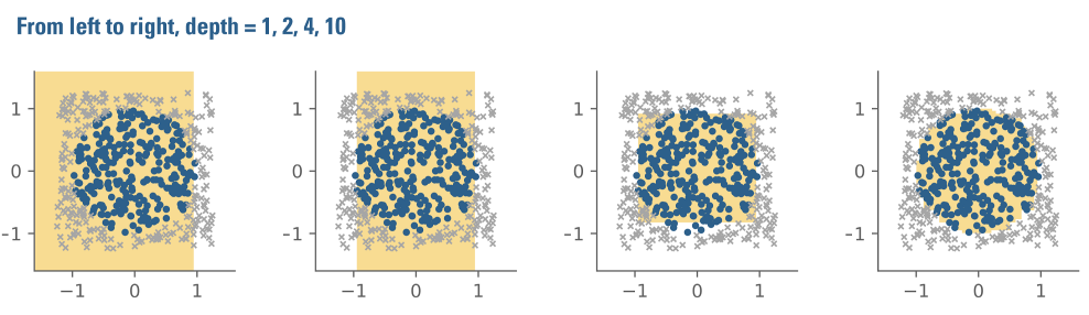
Figure A3 illustrates the workings of a decision tree in the context of the circle problem. If we could only pose one question, the best we could do in guessing whether an observation is inside or outside the circle, i.e., blue or grey, might be to check whether its x coordinate is larger than some number close to 1. That’s because any datapoint whose x coordinate is greater than 1 must lie outside the circle. This is evident in Figure A1: no points to the right of 1 are blue.

The leftmost plot in Figure A3 illustrates the  result of applying this rule. Points guessed to be inside the circle are represented by the yellow shaded area.  Points guessed to lie outside of the circle lie in the unshaded region.

When allowed to ask only one question, the algorithm’s predictive accuracy is terrible: the yellow shaded area looks nothing like a circle.

But by asking successively more questions about the data, looking from left to right, the yellow-shaded approximation improves. At a depth of 10, on the far right, it looks quite good.

Figure A2: A hypothetical "20-questions" decision tree for guessing an animal

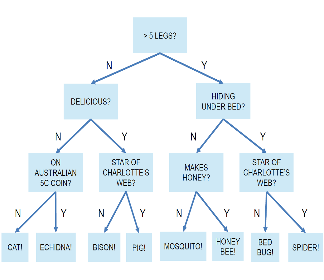
Figure A3: Decision tree accuracy as a function of tree "depth"

In general, decision trees are constructed in this step by-step manner. The algorithm starts by identifying an inpidual feature and an associated value that, in isolation from all the other features, most accurately classifies the datapoints. The process is then repeated within each of the two resulting subsamples, and so on, until the tree reaches a preset limit on its depth or some other stopping criterion set by the researcher.

This stepwise approach to tree construction is termed a “greedy” algorithm. Greedy is technical jargon indicating that at each stage of the tree the algorithm selects a feature and a value based only on the immediate improvement in classification without considering implications further down the tree. We would expect superior classification ability from a holistic approach that simultaneously considers the combined effect of all subsequent feature and value selections. Unfortunately, such algorithms are often computationally infeasible.

This step-by-step tree construction approach has a visibly interesting consequence in the context of the circle problem. Because the algorithm only considers one feature at a time, either x or y, every line drawn must be parallel to either the y or the x-axis. This is easy to see in the three left-most panels of Figure A3. As we allow the tree to have greater depth, i.e., as we ask more and more questions, the boundary appears more and more circular. But squinting at the image reveals that the circle approximation still consists only of lines parallel to either the x- and y-axis. The broader point is that understanding how an algorithm works can help to provide a sense of the complexity required to accomplish a particular task.

Support Vector Machines

While Support Vector Machines (SVM) have a complex name, they are an intuitive method of classifying data. The circle problem is ideally suited to illustrating how they work.

In this context, the key question is whether we can distinguish points inside and outside of a circle with a straight line. (This property is known as “linear separability.”) Unfortunately, this doesn’t look possible even from just a cursory glance at Figure A1. Why do we care? Because it’s easier to work with and to fit straight lines than curves. This concept becomes increasingly important as the complexity of the data increases, i.e., as we have more and more features.

It turns out, though, that by transforming the information in each data point’s x and y values, we might be able to do it. Specifically, we could create two new features, x² and y². If we then re-chart the datapoints on the basis of those transformed (squared) values we get Figure A4. It’s clear in this picture that the blue and grey points are now separable by the green straight line. ⁸ 

Figure A4: The circle data set transformed

To generalize from the circle example, SVMs find transformations of data, specifically new “coordinate systems,” that make classifying the data easier. Through resource efficient computer implementations, they can try hundreds of alternatives, starting with small powers of the original features, squares and cubes, and progressively larger and larger ones. The algorithm will then choose the transformation and classification rule that best separates the two groups of data. 

Neural Networks

Artificial neural networks (commonly just “neural networks”) are the most flexible of the three methods. They can approximate intricate functional relationships in data. The cost of this flexibility is algorithmic and computational complexity and opacity.

Neural networks are based on the behavior of neurons in the human brain. Roughly speaking, neurons receive and transmit chemical stimuli. They respond if the input stimulus exceeds a threshold level, at which point they transmit other chemicals to the next neuron in the chain. Artificial neurons seek to replicate this behavior as shown in the top row of Figure A5.

Neural networks are comprised of artificial neurons much like brains are comprised of biological neurons.  Figure A5 displays a generic schematic in which each white circle is such an artificial neuron. The researcher specifies what the nodes do and how they are arranged based on the nature of the problem at hand.

Instead of chemicals, artificial neural networks filter, process, and transform data. Features from the input dataset are passed into the first layer of nodes. If the data item received at a particular input node exceeds a certain threshold value, then the node will pass that information along to a node or several nodes in the next layer. A node may transform the data that it receives. It may combine information from several nodes in the prior layer, applying different weights to different sources. A neural network composed of several layers and a large number of nodes may extensively transform the data, abstracting it considerably away from the input information. This is how “deep learning” neural networks make complex decisions.

To implement a neural network, the researcher must specify its architecture, which is an engineering problem. The researcher sets 1) the number of layers of nodes, 2) which nodes are connected to each other, and 3) what transformation function is embedded in each node. In principle, a linear regression could be implemented as a simple neural network: it would consist of one layer, one node, and a regression line as the function (intercept + slope*input feature). In the training stage, the algorithm would estimate the regression intercept and slope to minimize the prediction error.

Figure A5: Neural network

Generally speaking, though, most networks employ functions that have an “on/off” property, resembling the firing of biological neuron. Perhaps for the largest input values the function would pass along a 1, for most other values a 0, and for a small range of values some number(s) between 0 and 1. Image recognition might provide an intuitive functional context: a neural network could take in a set of input features, e.g., pixels of from photos, and through the training process discriminate shading or coloration in which pixel locations, or combinations thereof, are predictively valuable in recognizing image types. Returning to the circle problem, Figure A6 compares classification ability of multiple neural network architectures where the functions at each node have the on/off property. Several architectures with modest numbers of parameters, i.e., only a few layers and nodes, do quite well at approximating the circle.

Figure A6: Classification ability of several neural network architectures

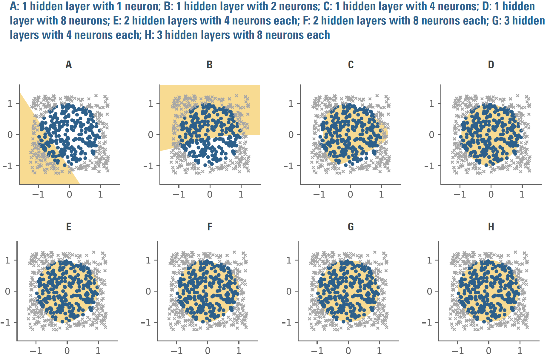
But even in this simple context, the opacity of these neural networks is problematic in trying to understand what they’re doing. Knowing the function of an inpidual node won’t provide much insight. The transparent flow of a decision tree or the nature of the data transformation applied by an SVM doesn’t have a clear analogue. What’s more, the number of parameters to estimate will grow rapidly as network architecture becomes richer, potentially consuming substantial data and computational expense in the training process.