Managed Volatility: Distinctively Different
Table of contents
Is managed volatility just value investing in disguise? No. Managed volatility is a fundamentally different strategy that is complementary to, not a substitute for, value approaches. Acadian’s Managed Volatility strategy invests in stocks that, in combination at the portfolio level, have experienced low levels of historical volatility and takes advantage of past failures of market prices to link risk to return. In a classic sense, this is a “value” approach. However, we have found compelling evidence that the two strategies offer unique characteristics and results that cannot be explained by their conventional factor exposures.
For more than 40 years, portfolios comprised of low-risk stocks have substantially outperformed their higher-risk counterparts. This anomaly runs counter to traditional finance theory, which predicts that increased risk will be rewarded by higher expected return. Managed volatility strategies are designed to take advantage of this mispricing. Their objective is to deliver equity returns with substantially lower risk. This gives rise to two possible theories. One is that managed volatility is simply value investing in disguise. The other is that managed volatility is a fundamentally different approach to investing.
Our results, based on U.S. data (the CRSP value-weighted U.S. index), show that managed volatility and conventional active value strategies appear to be distinct in important ways. Though in the past both have delivered better-than-market risk-adjusted returns, the strategies have low correlation with each other.1 Moreover, while conventional active strategies can explain a portion of the historic returns realized by managed volatility, there is an important component of managed volatility’s historic returns that appears to be unrelated to conventional active strategies.
Comparing Conventional Active Strategies to Managed Volatility
Active investing comes in many forms. For example, a famous value strategy advises buying stocks with low scaled-price ratios such as price/book or price/earnings. Such value strategies have typically outperformed the aggregate market. Other strategies that are not value strategies per se, but that are related to value, also have attracted attention. For example, some investors advise purchasing dividend-paying stocks at low prices: that is, buying stocks with high dividend yields. Such yield strategies also have outperformed the aggregate market. In another well-known approach, some investors buy small stocks, those with low market capitalizations. Consistent with this approach, the historical performance of size strategies also has been better than the market’s.
To highlight the difference between these conventional active strategies and managed volatility, we compare the historical monthly return series of four active hypothetical portfolios and the market for the period 1991 to 2015. The five hypothetical portfolios are:
- a value strategy consisting of a value-weighted allocation to stocks in the highest book-to-market quintile (Fama and French 1992);
- a size strategy consisting of a value-weighted allocation to stocks in the lowest market capitalization quintile (Fama and French 1992);
- a yield strategy consisting of a value-weighted allocation to stocks in the highest quintile of dividend yield (Naranjo et al. 1998);
- a minimum variance portfolio (Baker et al. 2011); and
- the aggregate market portfolio.
Figure 1 displays the historic buy-and-hold returns of the hypothetical portfolios representing the four conventional active strategies, as well as the aggregate market portfolio. In this example, the value, size, and yield portfolios each outperformed the market. Managed volatility, here represented by a minimum variance portfolio, also had a cumulative return greater than the market’s. Importantly, and readily apparent in Figure 1, managed volatility’s returns were much less volatile than the returns of all the conventional active strategies and also less volatile than the market’s returns. (More precisely, managed volatility has a Sharpe ratio for this period that is greater than the Sharpe ratios of value, size, yield, and the aggregate market. See Figure 1.) For example, the cumulative hypothetical return of managed volatility was roughly equal to the hypothetical returns of all these conventional strategies for the period 1991-2015 (and the sub-periods 1991-2002, 2002-2008, and 2009-2015) with far less volatility.
Figure 1
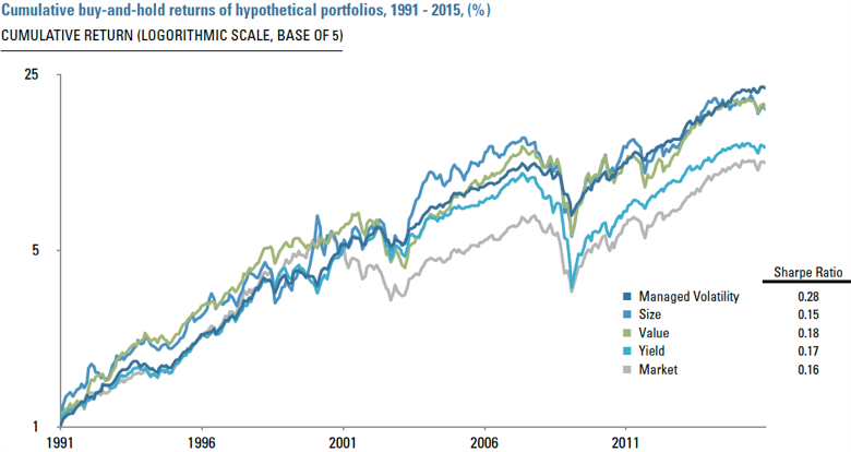
Figure 2
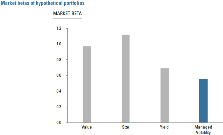
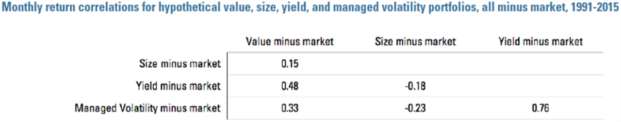
The hypothetical managed volatility portfolio’s high Sharpe ratio is a consequence of its better-than-market average returns combined with less-than-market risk.2 Another formal measure of risk is market beta: Figure 2 compares betas of the four active strategies. By design, managed volatility has far lower beta than the other three. Managed volatility’s low beta is in part due to its low correlation with the market; Figure 3 compares the market correlations of the four hypothetical portfolios. Correlations can also help characterize the relationships between these active strategies, and these measures provide further points of distinction. For excess returns over the risk-free rate, the correlations among the portfolios are high, but these statistics merely reflect the fact that any two long-only strategies in U.S. equities can display a relatively high correlation with the market and with each other. A more meaningful statistic is the correlation between two strategies once the common market component is subtracted. Table 1 displays these correlations. Once the common market component is subtracted, value and managed volatility exhibit a low correlation of 0.33. Similarly, size and managed volatility exhibit a negative correlation of -0.23. Managed volatility and yield are more highly, but still very imperfectly, correlated at 0.76. By these measures as well, each of the four hypothetical portfolios is distinct from the others.
Figure 3
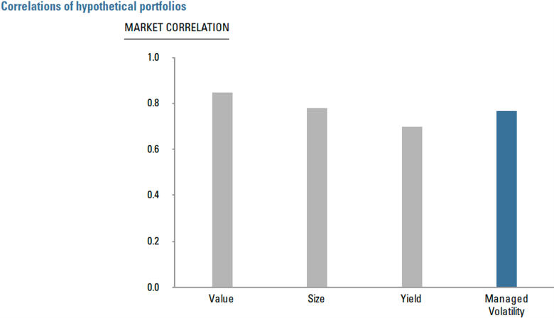
Table 1
Do Conventional Strategies Explain the Performance of Managed Volatility?
There is another way to assess whether or not managed volatility’s exposure to conventional active strategies explains its favorable historical returns. Researchers have developed a formal methodology for assessing any particular strategy’s relationship to characteristics such as value, size, and yield that historically have been associated with high average returns. Table 2 presents results of such tests for the four active hypothetical long-only portfolios. The left hand side of Table 2 lists factors for the aggregate market (MKT), value (HML), size (SMB) (Fama and French 1993), price momentum (MOM) (Carhart 1997),3 and yield (PMN: payer-minus-non-payer). The methodology removes the contributions of these factors from the hypothetical returns of the four portfolios.
Table 2
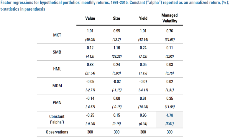
The row labeled Constant near the bottom of the table is the factor-adjusted alpha for each regression: it indicates the average return in each hypothetical portfolio that is not explained by the characteristic factors. For example the value factor (HML) explains much of the value portfolio’s return, so that after accounting for its contribution, the residual return is essentially zero (–25 basis points per year). This result demonstrates that the technique works the way we would like it to: the value factor fully explains the historic returns to the value portfolio. Similarly, the size factor (SMB) fully explains the historic returns to the size portfolio, leaving a minimal residual return (15 basis points per year). A similar result holds for the yield portfolio: the residual return is 96 basis points per year after removing the return explained by the yield (PMN) factor. However, the residual return of managed volatility behaves differently. After accounting for value, size, momentum, and yield factors, the residual return is both high and significant at 478 basis points per year on average (t-statistic 5.01).4 The result of this analysis of our hypothetical portfolios suggests that managed volatility exploits mispricings that are distinct from those exploited by the conventional strategies.
Summary
Conventional active strategies and managed volatility all take advantage of market mispricings, and each has offered an enhancement compared to the aggregate market. However, the strategies differ in important ways. Their excess-to-market returns have low correlation, suggesting that they are indeed different strategies. Managed volatility’s Sharpe ratio is higher than those of the conventional strategies, suggesting that even if managed volatility were taking advantage of precisely the same mispricings as the conventional active strategies, managed volatility offers a better implementation. However, the evidence suggests that managed volatility is not exploiting exactly the same mispricings as the conventional active strategies, because, at least for recent decades, conventional factors cannot explain managed volatility’s excess return.
Because of its high Sharpe ratio, its low correlation with conventional active strategies, and its unique sources of excess return, managed volatility may be considered a distinct and beneficial addition to an investment portfolio that employs standard tracking-error-minimizing strategies, even value. Investing in both conventional active strategies and a managed volatility strategy may provide useful diversification and an improved Sharpe ratio relative to investing only in one.
References
Baker, Malcolm, Brendan Bradley, and Jeffrey Wurgler, “Benchmarks as Limits to Arbitrage: Understanding the Low-Volatility Anomaly,” Financial Analysts Journal 67, no.1, 2011, 40-54.
Carhart, Mark M., “On Persistence in Mutual Fund Performance,” Journal of Finance, vol.52, March 1997, 57-82.
Fama, Eugene F. and Kenneth French, “The Cross-Section of Expected Stock Returns,” Journal of Finance vol. 47, 1992, 427-465.
Fama, Eugene F. and Kenneth French, “Common Risk Factors in the Returns of Bonds and Stocks,” Journal of Financial Economics 33, 1993, 3-56.
Naranjo, Andy, M. Nimalendran, and Mike Ryngaert, “Stock Returns, Dividend Yields, and Taxes,” Journal of Finance no. 53 (6), 1998, 2029-2057.
Pastor, Lubos and Robert F. Stambaugh, “Liquidity Risk and Expected Stock Returns,” Journal of Political Economy 111 (3), 2003, 642-685.
Endnotes
- In this paper, use of the past tense indicates a statement about historical facts. Under no circumstances should such statements be interpreted as predictions of the future. Past performance is not indicative of future results.
- In fact, the Sharpe ratios in Figure 1 likely understate the performance difference between managed volatility and conventional strategies, because the difference between historical average returns and historical realized cumulative returns will be greater for the conventional strategies as a consequence of their higher volatility.
- The momentum factor is commonly included in factor regressions, so for consistency we included it here. However, the price momentum strategy, the buying of stocks with high past returns and the selling of stocks with low past returns, is distinct from the other active strategies discussed in this paper, because it is not based on a current or past price as are the others, but instead is based on a past return.
- The result is unchanged if the Pastor-Stambaugh (2003) liquidity factor, which has zero loading and no significance in these regressions, is added to the right-hand side.
Hypothetical Legal Disclaimer
Acadian is providing hypothetical performance information for your review as we believe you have access to resources to independently analyze this information and have the financial expertise to understand the risks and limitations of the presentation of hypothetical performance. Please immediately advise if that is not the case.
Hypothetical performance results have many inherent limitations, some of which are described below. No representation is being made that any account will or is likely to achieve profits or losses similar to those shown. In fact, there are frequently sharp differences between hypothetical performance results and the actual performance results subsequently achieved by any particular trading program.
One of the limitations of hypothetical performance results is that they are generally prepared with the benefit of hindsight. In addition, hypothetical trading does not involve financial risk, and no hypothetical trading record can completely account for the impact of financial risk in actual trading. For example, the ability to withstand losses or to adhere to a particular trading program in spite of trading losses are material points which can also adversely affect actual trading results. There are numerous other factors related to the markets in general or to the implementation of any specific trading program which cannot be fully accounted for in the preparation of hypothetical performance results and all of which can adversely affect actual trading results.
Legal Disclaimer
These materials provided herein may contain material, non-public information within the meaning of the United States Federal Securities Laws with respect to Acadian Asset Management LLC, Acadian Asset Management Inc. and/or their respective subsidiaries and affiliated entities. The recipient of these materials agrees that it will not use any confidential information that may be contained herein to execute or recommend transactions in securities. The recipient further acknowledges that it is aware that United States Federal and State securities laws prohibit any person or entity who has material, non-public information about a publicly-traded company from purchasing or selling securities of such company, or from communicating such information to any other person or entity under circumstances in which it is reasonably foreseeable that such person or entity is likely to sell or purchase such securities.
Acadian provides this material as a general overview of the firm, our processes and our investment capabilities. It has been provided for informational purposes only. It does not constitute or form part of any offer to issue or sell, or any solicitation of any offer to subscribe or to purchase, shares, units or other interests in investments that may be referred to herein and must not be construed as investment or financial product advice. Acadian has not considered any reader's financial situation, objective or needs in providing the relevant information.
The value of investments may fall as well as rise and you may not get back your original investment. Past performance is not necessarily a guide to future performance or returns. Acadian has taken all reasonable care to ensure that the information contained in this material is accurate at the time of its distribution, no representation or warranty, express or implied, is made as to the accuracy, reliability or completeness of such information.
This material contains privileged and confidential information and is intended only for the recipient/s. Any distribution, reproduction or other use of this presentation by recipients is strictly prohibited. If you are not the intended recipient and this presentation has been sent or passed on to you in error, please contact us immediately. Confidentiality and privilege are not lost by this presentation having been sent or passed on to you in error.
Acadian’s quantitative investment process is supported by extensive proprietary computer code. Acadian’s researchers, software developers, and IT teams follow a structured design, development, testing, change control, and review processes during the development of its systems and the implementation within our investment process. These controls and their effectiveness are subject to regular internal reviews, at least annual independent review by our SOC1 auditor. However, despite these extensive controls it is possible that errors may occur in coding and within the investment process, as is the case with any complex software or data-driven model, and no guarantee or warranty can be provided that any quantitative investment model is completely free of errors. Any such errors could have a negative impact on investment results. We have in place control systems and processes which are intended to identify in a timely manner any such errors which would have a material impact on the investment process.
Acadian Asset Management LLC has wholly owned affiliates located in London, Singapore, and Sydney. Pursuant to the terms of service level agreements with each affiliate, employees of Acadian Asset Management LLC may provide certain services on behalf of each affiliate and employees of each affiliate may provide certain administrative services, including marketing and client service, on behalf of Acadian Asset Management LLC.
Acadian Asset Management LLC is registered as an investment adviser with the U.S. Securities and Exchange Commission. Registration of an investment adviser does not imply any level of skill or training.
Acadian Asset Management (Singapore) Pte Ltd, (Registration Number: 199902125D) is licensed by the Monetary Authority of Singapore. It is also registered as an investment adviser with the U.S. Securities and Exchange Commission.
Acadian Asset Management (Australia) Limited (ABN 41 114 200 127) is the holder of Australian financial services license number 291872 ("AFSL"). It is also registered as an investment adviser with the U.S. Securities and Exchange Commission. Under the terms of its AFSL, Acadian Asset Management (Australia) Limited is limited to providing the financial services under its license to wholesale clients only. This marketing material is not to be provided to retail clients.
Acadian Asset Management (UK) Limited is authorized and regulated by the Financial Conduct Authority ('the FCA') and is a limited liability company incorporated in England and Wales with company number 05644066. Acadian Asset Management (UK) Limited will only make this material available to Professional Clients and Eligible Counterparties as defined by the FCA under the Markets in Financial Instruments Directive, or to Qualified Investors in Switzerland as defined in the Collective Investment Schemes Act, as applicable.